6.3.7. 2-D Maxwell training-data generation

Solver-neutral Maxwell contracts solves one 2-D Maxwell problem at a time. Training a network needs many, spanning a distribution of plausible geology, converted into the same shape every later stage agrees on. generate_2d_maxwell_dataset() is that bridge: it draws a correlated resistivity field from geology for each realization, solves it with MT2DAdapter through solve_batch() (cached and retried rather than resolved from scratch on every call), and packages every realization that converges into a Maxwell2DDataset with a realization-level train/validation/test split and a DatasetManifest. A realization whose solve does not converge is recorded and excluded, never silently included.

The generator is best understood as four linked contracts rather than one large function call: a geological field defines the target, a solver mesh and receiver layout define the forward problem, canonical SurveyData defines the response axes, and the split plus manifest define which accepted realizations may be used for each statistical role. A dataset is ready for training only when all four contracts have been reviewed.

6.3.7.1. Configuring one coherent dataset

A Maxwell2DDatasetConfig fixes everything that must stay identical across realizations for the dataset to be one coherent, versioned thing: the shared (z, x) GeologyGrid, the horizontal and vertical correlation-length ranges realizations are drawn from, the shared frequency grid and receiver x positions, and a root Random seed from which every realization’s field and solver seeds are derived deterministically:

>>> from pycsamt.ai.geology import GeologyGrid
>>> from pycsamt.ai.training.dataset2d import (
...     Maxwell2DDatasetConfig,
...     generate_2d_maxwell_dataset,
... )

>>> grid = GeologyGrid.regular_2d(nx=6, nz=4, dx_m=300, dz_m=150)
>>> config = Maxwell2DDatasetConfig(
...     dataset_id="demo-2d-v1",
...     grid=grid,
...     correlation_length_x_m=(600.0, 900.0),
...     correlation_length_z_m=(150.0, 300.0),
...     frequencies_hz=[10.0, 3.0],
...     station_x_m=[600.0, 900.0, 1200.0],
...     n_realizations=2,
...     seed=0,
...     validation_fraction=0.0,
...     test_fraction=0.0,
... )
>>> config.components
('zxy', 'zyx')
>>> config.grid.shape, config.station_x_m.shape
((4, 6), (3,))
>>> config.to_dict()["schema_version"]
1

>>> dataset = generate_2d_maxwell_dataset(config)
>>> len(dataset.samples), dataset.rejected
(2, ())

Every accepted realization comes back as a Maxwell2DSample pairing the true resistivity grid (the training target) with its simulated SurveyData response (the training input) and the solver’s own mesh size and residual, so a downstream consumer never has to guess how well that one realization actually converged:

>>> sample = dataset.samples[0]
>>> sample.survey.shape
(3, 2, 2)
>>> sample.resistivity_ohm_m.shape
(4, 6)
>>> sample.mesh_cells, round(sample.relative_residual, 6)
(8650, 0.0)
>>> f"{sample.relative_residual:.3e}"
'2.290e-17'

Two realizations, three stations, two frequencies, and both impedance components finish quickly here because the mesh and realization count are kept deliberately small for the documentation build; the mesh alone uses 8,650 padded cells even at this scale, which is why Solver-neutral Maxwell contracts’s cache and batch runner, not a plain loop, are what make a production-sized version of this call tractable. Rounding the residual to six decimals hides its magnitude, which is why the scientific-notation output is also captured. The \(2.290\times10^{-17}\) residual shows an accurate solution of the discretized linear system; it does not prove that the mesh is sufficiently refined or that its boundaries are far enough away. The empty rejected tuple shows that neither attempted realization was excluded.

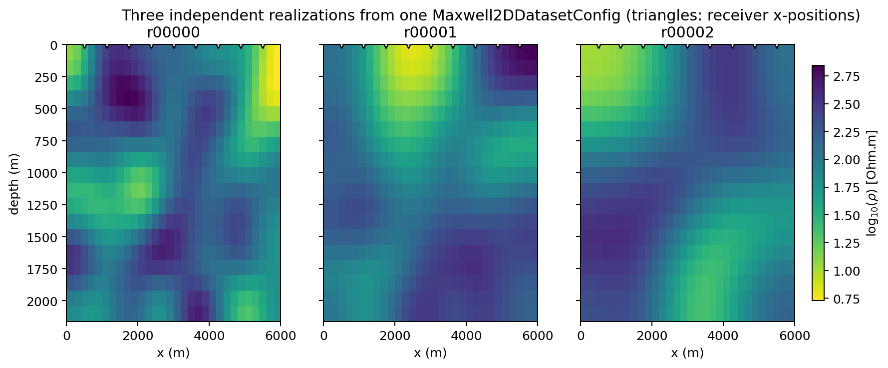
Three realizations drawn from the same Maxwell2DDatasetConfig — same correlation-length ranges, same station layout (white triangles), independent random fields. Each is a genuinely 2-D section with structure varying in both x and z, not a set of independent 1-D columns tiled side by side; that lateral continuity is the entire reason this module exists rather than reusing Forward Modelling’s station-wise 1-D batch generator.

The gallery should be read horizontally. All panels share one color scale, so the purple shallow resistor in the left realization is genuinely more resistive than the green material in the right panel rather than an artifact of independently stretched color limits. The correlation ranges impose broad smooth bodies; they do not create discrete contacts or faults. A network trained only on this family will therefore be biased toward smooth recovery even if its architecture contains no explicit smoothness penalty.

6.3.7.2. From complex impedance to network channels

The solver returns SI impedance in V/A with canonical shape (station, frequency, component). Apparent resistivity and phase are derived without changing that provenance:

(1)\[\rho_a^{(c)}(s,f)= \frac{|Z_c(s,f)|^2}{\mu_0\,2\pi f}, \qquad \phi^{(c)}(s,f)=\operatorname{atan2} \left(\Im Z_c,\Re Z_c\right).\]

Equation (1) is the SI conversion. The legacy \(0.2|Z|^2/f\) factor belongs to impedance expressed in mV/km/nT and must not be applied directly to the Maxwell adapter’s V/A output. For U-Net training, pyCSAMT uses \(\log_{10}\rho_a^{xy}\) and \(\phi^{xy}\) as its current two-channel layout, then transposes the arrays to (realization, channel, frequency, station).

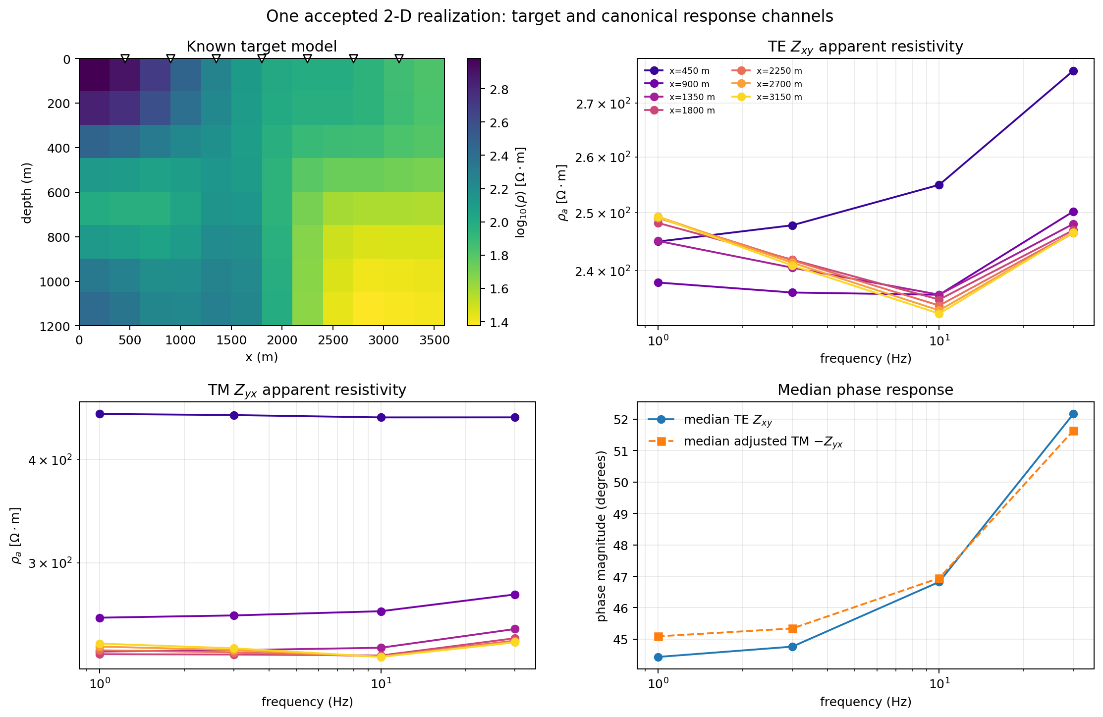
One accepted deterministic realization. White triangles identify the seven receiver positions. The upper-right and lower-left panels use identical station colors, letting a reader trace how the same lateral location differs between TE and TM. The phase panel plots \(-Z_{yx}\) for TM so its half-space reference is near \(+45^\circ\), consistent with the standard \(Z_{yx}=-Z_{xy}\) convention.

The target contains a shallow resistive zone on the left and a deeper conductive region toward the right. TE apparent resistivity varies moderately among most stations but rises most strongly at the leftmost receiver, which is consistent with its proximity to the shallow resistor. TM shows a larger separation at the same receiver because lateral conductivity enters its governing diffusion coefficient. This is a qualitative consistency check, not an inversion: the plotted response is still influenced by the full model, frequency-dependent sensitivity, mesh, and boundary conditions. Notice also that four frequencies cannot resolve every one of the 96 target cells; the target grid describes what was generated, not what those responses uniquely identify.

6.3.7.3. Two impedance modes, and why one needed more care than the other

A 2-D MT problem separates into two independent modes, and they are not equally easy to discretize. With \(\mu=\mu_0\) constant everywhere, TE mode solves for the electric field \(E_y\) under

(2)\[\nabla^2 E_y = i\omega\mu_0\sigma\,E_y,\]

a constant-coefficient Laplacian: resistivity structure enters only through the reaction term on the right, multiplying the field itself rather than its derivatives. TM mode solves for the magnetic field \(H_y\) under

(3)\[\nabla\cdot(\rho\,\nabla H_y) = i\omega\mu_0 H_y,\]

where resistivity sits inside the derivative — the diffusion coefficient itself, not just a multiplier. Equation (3) is a genuinely harder numerical problem than (2): every bit of 2-D resistivity structure a finite-difference scheme needs to resolve has to survive being differentiated through, not just multiplied in afterward. In practice this means TM mode needs finer joint horizontal and vertical resolution than TE mode to reach comparable accuracy — and that requirement, not a defect in the solver, was the real story behind an earlier, mistaken finding that TM mode was unusable for laterally fine structure. That investigation changed horizontal and vertical resolution one at a time instead of together, and compared independent random-field realizations across different resolutions instead of refining one fixed field — both of which produce exactly the appearance of a solver that never converges, even when it does. Once resolution is refined in both directions together on one fixed field, TM mode converges cleanly, changing by under 1-2% between realistic production resolution and twice that.

A second, real but smaller issue was fixed alongside that finding: pycsamt.forward.em2d’s TM-mode assembly combined resistivity values at cell interfaces with a plain arithmetic mean, which is the correct combination for two cells in series along the direction being differentiated but not for the two cells actually involved here, which act as parallel current paths. The physically correct combination — a thickness-weighted harmonic mean of resistivity — is what the surface-response extraction already used; the interior assembly now matches it. Both impedance modes are therefore validated and requested by default, and a near-uniform model confirms both against the analytic half-space limit at once:

>>> import numpy as np
>>> from pycsamt.forward.maxwell.benchmarks import half_space_impedance

>>> grid = GeologyGrid.regular_2d(nx=4, nz=4, dx_m=200, dz_m=100)
>>> config = Maxwell2DDatasetConfig(
...     dataset_id="halfspace-check",
...     grid=grid,
...     correlation_length_x_m=(1.0, 2.0),
...     correlation_length_z_m=(1.0, 2.0),
...     frequencies_hz=[10.0, 1.0],
...     station_x_m=[400.0],
...     n_realizations=1,
...     seed=0,
...     log_resistivity_mean=2.0,
...     log_resistivity_std=1e-6,
...     validation_fraction=0.0,
...     test_fraction=0.0,
... )
>>> dataset = generate_2d_maxwell_dataset(config)
>>> sample = dataset.samples[0]
>>> analytic = half_space_impedance(100.0, config.frequencies_hz)
>>> zxy = sample.survey.impedance[0, :, 0]
>>> zyx = sample.survey.impedance[0, :, 1]
>>> te_error = np.abs(zxy - analytic) / np.abs(analytic)
>>> round(float(np.max(te_error)), 4)
0.0424

>>> # Zyx = -Zxy for an isotropic half-space (standard MT convention).
>>> tm_error = np.abs(zyx - (-analytic)) / np.abs(analytic)
>>> round(float(np.max(tm_error)), 4)
0.0411

Both modes agree with the analytic reference to about 4%, using this module’s own default mesh construction rather than a specially tuned one — the same order of accuracy for both, not TE working and TM silently failing next to it.

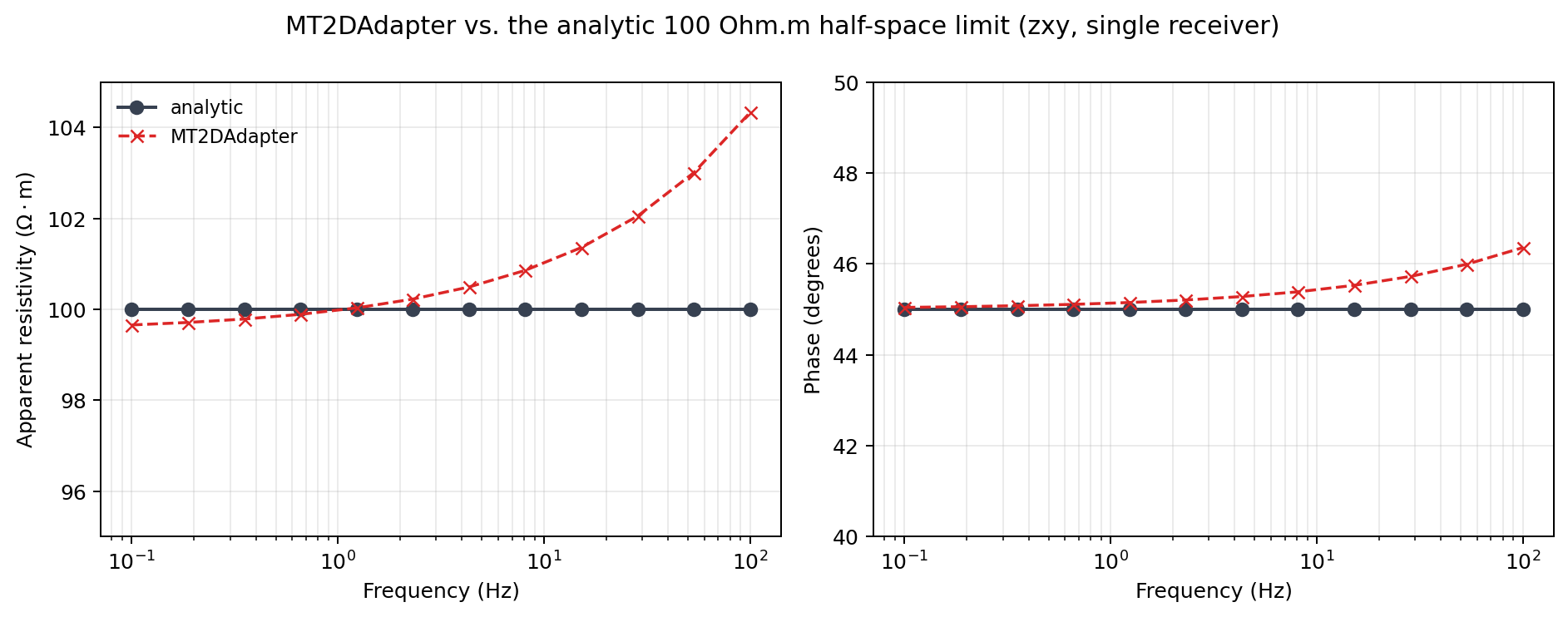
The numerical curve remains close to the analytic 100 \(\Omega\,m\) response and \(45^\circ\) phase over frequency. This panel displays TE; the captured numbers above provide the corresponding TM error check. A half-space benchmark detects unit, sign, boundary, and gross discretization faults, but heterogeneous refinement tests are still required because a uniform earth cannot exercise interface averaging.

6.3.7.4. Fail fast before an impractical mesh

The lateral mesh remains uniform because graded lateral cells were found to damage TM accuracy. Consequently a low frequency, high resistivity, fine dx_m, or large mesh_safety_factor can request too many cells. The max_mesh_cells guard reports the required domain instead of silently coarsening the physics:

>>> guard_grid = GeologyGrid.regular_2d(
...     nx=6, nz=4, dx_m=300.0, dz_m=150.0
... )
>>> guarded = Maxwell2DDatasetConfig(
...     dataset_id="guard-demo",
...     grid=guard_grid,
...     correlation_length_x_m=(600.0, 900.0),
...     correlation_length_z_m=(150.0, 300.0),
...     frequencies_hz=[10.0, 3.0],
...     station_x_m=[600.0, 900.0, 1200.0],
...     n_realizations=1,
...     seed=0,
...     max_mesh_cells=2,
...     validation_fraction=0.0,
...     test_fraction=0.0,
... )
>>> try:
...     generate_2d_maxwell_dataset(guarded)
... except ValueError as exc:
...     print(str(exc).split(". ", 1)[0] + ".")
requested configuration needs 312 uniform x-cells (lateral extent 93415 m at 300 m resolution), exceeding max_mesh_cells=2.

Do not respond automatically by raising the cap. First decide whether the frequency band, resistivity prior, spatial resolution, and safety factor are scientifically required. If they are, estimate memory and runtime explicitly; if they are not, revise the configuration and record why. Coarsening dx_m changes both the geological target and the numerical approximation.

6.3.7.5. Handing this to noise, or to training

This module deliberately stops at a clean, forward-consistent response. Turning it into training data that resembles a specific field survey — adding heteroscedastic noise, dropout, static shift, and distortion fitted from that survey’s own quality control — is Domain-gap and noise simulation’s job, kept separate so that a clean control dataset always exists independently of whatever noise model is layered on top of it. From there, a Maxwell2DDataset’s train/ validation/test partitions and its DatasetManifest are exactly the inputs Loss functions for scientific inversion trains against and Recovery, residual, and OOD diagnostics reports evidence from — the realization-level split guarding against the same leakage Canonical data contracts already enforces for any other kind of split.

The two-realization example deliberately has no held-out samples. A training corpus should make the partition sizes explicit before any solve budget is committed:

>>> plan_grid = GeologyGrid.regular_2d(
...     nx=8, nz=8, dx_m=300.0, dz_m=150.0
... )
>>> production_plan = Maxwell2DDatasetConfig(
...     dataset_id="profile-2d-v2",
...     grid=plan_grid,
...     correlation_length_x_m=(600.0, 1500.0),
...     correlation_length_z_m=(150.0, 450.0),
...     frequencies_hz=[30.0, 10.0, 3.0, 1.0],
...     station_x_m=[300.0, 600.0, 900.0, 1200.0],
...     n_realizations=100,
...     seed=42,
...     validation_fraction=0.15,
...     test_fraction=0.15,
... )
>>> production_plan.n_realizations
100
>>> production_plan.validation_fraction, production_plan.test_fraction
(0.15, 0.15)

This is a configuration example, not a claim that 100 realizations are adequate. Adequacy depends on geological diversity, target dimension, rejection rate, nuisance variants, and the precision required for scenario- specific validation. After generation, inspect dataset.split.sizes rather than inferring counts from fractions, because rejected solves are removed before splitting. Persist dataset.manifest and link later noise variants to each clean realization_id so no parent model crosses partitions.