
8.2. Lithology classification#
Interpretation workflow treats “calibrate and classify the model” as a single step:
pycsamt.interp.ModelCalibrator blends borehole evidence into the
model and hands the result to pycsamt.geology.lithology.RockDatabase
for classification. This page opens that classification engine on its own,
using the same five-station fixture and station naming (S00-S04)
introduced in Interpretation workflow, so a resistivity value can be turned into a
lithology name without a calibrator, a borehole, or even a
ResistivityModel in the loop.
The classification engine itself lives in pycsamt.geology –
general geological domain knowledge with no electromagnetic dependency –
rather than in pycsamt.interp. RockDatabase and the other
classes below remain importable as pycsamt.interp.RockDatabase for
convenience, exactly as used throughout this guide.
A RockDatabase is an ordered collection of
RockEntry records, each naming a
\([\rho_{\min}, \rho_{\max}]\) resistivity range in ohm metres:
>>> from pycsamt.interp import RockDatabase

>>> db = RockDatabase.default()
>>> len(db)
49
>>> db
RockDatabase(49 entries)
8.2.1. Built-in rock database#
RockDatabase.default() returns entries from
pycsamt.geology.rock_library.BUILTIN_ROCKS, a literature-compiled
table (Palacky 1988; Telford, Geldart and Sheriff 1990; Keller and
Frischknecht 1966; Slichter and Telkes 1942) kept in its own module,
separate from the classification engine in this page, specifically so it
can keep growing – a contributor adding a regional ore mineral or a
cold-region lithology only ever touches
pycsamt.geology.rock_library. It currently holds 49 entries. Each
entry is a plain, inspectable record; the entries property returns them
as a read-only tuple in the order they were inserted, from the most
conductive to the most resistive:
>>> db.entries[0]
RockEntry(name='Sulfide ore body', rho_min=0.001, rho_max=0.1, color='#2C3E50', description='Massive sulfides, pyrite, chalcopyrite', code=1, source='Telford, Geldart & Sheriff (1990); Slichter & Telkes (1942)')
>>> db.entries[-1]
RockEntry(name='Amphibolite', rho_min=1000, rho_max=10000, color='#4A235A', description='Mafic-derived medium-to-high-grade metamorphic', code=49, source='Telford, Geldart & Sheriff (1990)')
code is the integer written to LAS exports (see Export and reporting);
color drives every lithology-aware plot in pycsamt.interp.plot;
source is the citation backing that specific range, worth carrying into
any exported table alongside the classification itself. Plotting every
range together, on a log resistivity axis, makes the database’s central
design choice visible:
>>> import matplotlib.pyplot as plt

>>> entries = sorted(db.entries, key=lambda e: e.rho_min)
>>> fig, ax = plt.subplots(figsize=(8, 9))
>>> for i, e in enumerate(entries):
...     _ = ax.barh(i, e.rho_max - e.rho_min, left=e.rho_min, height=0.7,
...                  color=e.color, edgecolor="0.3", linewidth=0.6)
...     _ = ax.plot(e.rho_mid, i, marker="|", color="black", markersize=10, mew=1.2)
>>> _ = ax.set_yticks(range(len(entries)))
>>> _ = ax.set_yticklabels([e.name for e in entries], fontsize=8)
>>> _ = ax.set_xscale("log")
>>> _ = ax.set_xlim(1e-3, 1e13)
>>> _ = ax.set_xlabel(r"Resistivity $\rho$ ($\Omega\,\mathrm{m}$, log scale)")
>>> _ = ax.set_title("RockDatabase.default() — built-in resistivity ranges")
>>> _ = ax.grid(axis="x", which="both", alpha=0.25)
>>> _ = ax.invert_yaxis()
>>> fig.tight_layout()
>>> fig.savefig("review/rock_database_ranges.png", dpi=200, bbox_inches="tight")
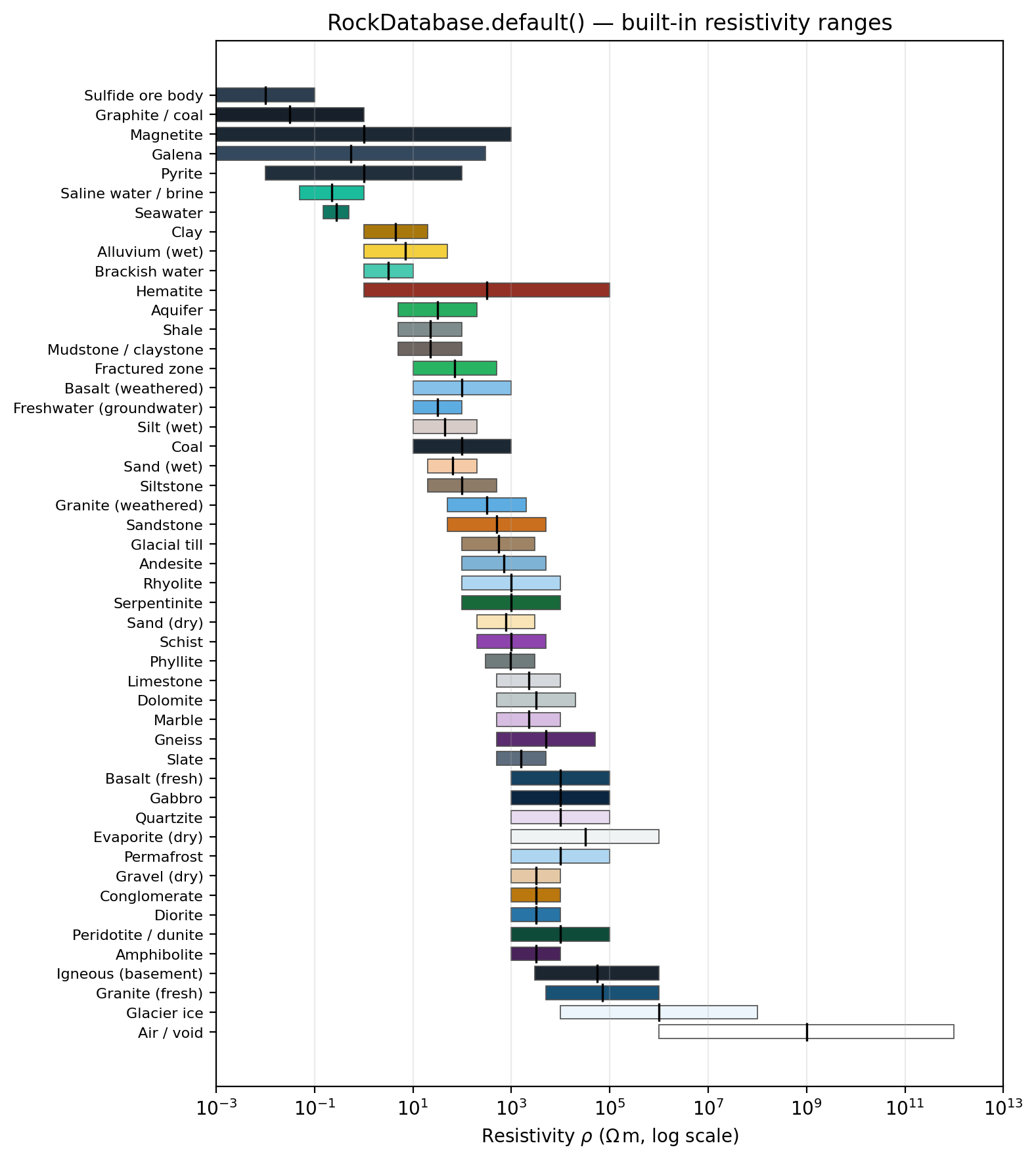
Every entry in RockDatabase.default(), ordered by rho_min. The
tick mark inside each bar is rho_mid, the geometric-mean midpoint used
for classification. Bars overlap across most of the chart: a single
resistivity value routinely falls inside four, five, or more named ranges
at once.#
That overlap is not a database defect. Sulfide mineralization, saline pore water, clay, and thin fracture zones can all present a few ohm metres; fresh granite, gabbro, and quartzite can all present tens of thousands of ohm metres. Resistivity constrains the plausible lithology set; it rarely narrows that set to one member without independent evidence, which is why Interpretation workflow treats database-only classification as a hypothesis to be checked against boreholes, not a measurement.
8.2.2. Nearest and overlap matching#
classify() resolves that overlap with two strategies, selected by
method. The default, nearest-midpoint classification, ignores
containment altogether and returns whichever entry’s rho_mid is closest
to the query in \(\log_{10}\) space. method="overlap" instead returns
the first entry, in database order, whose range actually contains the query.
Querying \(\rho=250\ \Omega\mathrm{m}\) – a value inside fifteen
different entries at once – shows them disagreeing:
>>> nearest = db.classify(250.0)
>>> overlap = db.classify(250.0, method="overlap")
>>> nearest.name, overlap.name
('Granite (weathered)', 'Fractured zone')
>>> nearest.contains(250.0), overlap.contains(250.0)
(True, True)
>>> [e.name for e in db.entries if e.contains(250.0)]
['Fractured zone', 'Granite (weathered)', 'Basalt (weathered)', 'Sand (dry)', 'Sandstone', 'Schist', 'Magnetite', 'Galena', 'Hematite', 'Glacial till', 'Siltstone', 'Coal', 'Andesite', 'Rhyolite', 'Serpentinite']
Both answers are defensible read from the database alone; they simply apply
different tie-breaking rules to the same ambiguity. "overlap" depends on
insertion order in BUILTIN_ROCKS, which
is not a geological ranking, so prefer it only when the database has been
curated so that earlier entries should win ties (for example, a locally
dominant unit placed first). The default "nearest" has no such order
dependency, which is why it is also
what classify_column() and
StratigraphicLog.from_column()
use internally – neither exposes a method argument, so every
StratigraphicLog in this guide, including the ones
built by ModelCalibrator in Interpretation workflow, is
classified with nearest-midpoint matching only.
8.2.3. Extrapolation and missing values#
classify() never raises. Two situations are worth knowing about before
they appear silently inside a station log.
Warning
classify(rho) returns the database’s first entry whenever rho is
nan, zero, or negative, without any warning:
>>> db.classify(float("nan")).name
'Sulfide ore body'
>>> db.classify(0.0).name
'Sulfide ore body'
>>> db.classify(-5.0).name
'Sulfide ore body'
In RockDatabase.default() that happens to be 'Sulfide ore body',
simply because it is first in
BUILTIN_ROCKS – it carries no
diagnostic meaning. Run the finite-value audit from Interpretation workflow
before classification, not after: a masked air cell or a bad log10
conversion that reaches classify_column unnoticed will be labelled as
sulfide ore rather than flagged.
Beyond the database’s own coverage (below \(10^{-3}\) or above
\(10^{12}\ \Omega\mathrm{m}\)), nearest-midpoint matching keeps returning
the closest edge entry even though that entry no longer contains the query –
this is the one situation where nearest and containment genuinely
disagree inside normal use:
>>> low, high = db.classify(1e-6), db.classify(1e13)
>>> low.name, low.contains(1e-6)
('Sulfide ore body', False)
>>> high.name, high.contains(1e13)
('Air / void', False)
Both values are outside anything a CSAMT, AMT, or MT survey should recover; seeing them in a classified log points back to a unit or grid problem upstream, not to a genuinely novel lithology.
8.2.4. Custom rock databases#
A project-specific database loads from CSV with
RockDatabase.from_csv().
Required columns are name, rho_min, rho_max; color,
description, and code are optional and default to a neutral grey, an
empty string, and the row’s 1-based position:
name,rho_min,rho_max,color,description,code
Laterite,80,600,#B5651D,Ferricrete duricrust,1
Saprolite,20,300,#C9A66B,Deeply weathered granite regolith,2
Fresh basement,3000,200000,#4A4A4A,Unweathered gneiss/granite basement,3
Loading this three-entry regional database and classifying the same profile from the built-in one:
>>> from pycsamt.interp import RockDatabase

>>> db_regional = RockDatabase.from_csv("configuration/rocks_regional.csv")
>>> len(db_regional)
3
>>> db_regional.classify(150.0).name
'Laterite'
Replacing the default database changes every downstream classification: the
same 150 ohm metre cell that was 'Basalt (weathered)' against the
built-in set becomes 'Laterite' against a three-entry regional
one, simply because there is no basalt entry to compete for the
nearest-midpoint match. Keep the database used for a given interpretation
recorded alongside its parameters – configuration/ in the project layout
from Interpretation workflow is exactly the place for it – because a station log is
only meaningful together with the database that produced it.
A rock database alone has no concept of depth or station position; it only
maps one resistivity value to one name at a time.
classify_column() applies
classify() to every cell in a \(\log_{10}(\rho)\) depth column, and
StratigraphicLog.from_column()
turns that per-cell labelling into depth intervals. Classifying station
S02’s raw, uncalibrated column directly – with no borehole and no
ModelCalibrator involved – gives:
>>> import numpy as np
>>> from pycsamt.interp import ResistivityModel, StratigraphicLog

>>> x_m = np.array([0.0, 250.0, 500.0, 750.0, 1000.0])
>>> z_m = np.array([5.0, 15.0, 30.0, 55.0, 90.0])
>>> rho_ohm_m = np.array([
...     [420, 380, 350, 410, 460],
...     [120,  95,  70, 110, 150],
...     [ 55,  42,  35,  48,  65],
...     [240, 190, 160, 210, 280],
...     [1800, 1500, 1200, 1650, 2100],
... ], dtype=float)
>>> model = ResistivityModel.from_array(
...     np.log10(rho_ohm_m), x_m, z_m,
...     station_x=x_m,
...     station_names=["S00", "S01", "S02", "S03", "S04"],
...     method="demonstration",
... )

>>> col02 = model.station_column("S02")
>>> [e.name for e in db.classify_column(col02)]
['Granite (weathered)', 'Fractured zone', 'Aquifer', 'Basalt (weathered)', 'Schist']

>>> log_db_only = StratigraphicLog.from_column("S02", 500.0, z_m, col02, db=db)
>>> len(log_db_only.layers)
5
Every cell here classifies to a different name, so nothing merges and the
log keeps all five model layers. Compare this against S02’s log in
Interpretation workflow, built from the calibrated model with BH01 in the loop:
four layers, headed by 'Sandstone' rather than 'Granite (weathered)'.
Nothing about the classification engine changed between the two; the
calibrator changed the resistivity values it was given first, by softly
matching nearby cells toward the borehole’s true resistivity. Database-only
classification of the calculated resistivity model and calibrated
classification of the borehole-adjusted model are different products with
different evidentiary weight, exactly as Interpretation workflow requires them to be
labelled.
8.2.5. Remote rock databases#
Every RockDatabase records where its
entries came from in metadata:
>>> db.metadata
{'origin': 'default'}
>>> db_regional.metadata["origin"]
'csv'
metadata["path"] for a CSV-loaded database stores the path as
str(Path(...)), so – exactly as with the exporter paths in
Interpretation workflow – it prints with native separators; compare it with
.as_posix() rather than a literal string when the comparison must be
platform-independent.
No public, machine-readable service currently maps a rock name to a
resistivity range the way BUILTIN_ROCKS
does – the literature it compiles is not something with a live API.
RockDatabase.from_url()
is built for a source you do control instead: a project or organisation
endpoint serving a JSON array with the same fields as RockEntry. It
caches successful responses under ~/.pycsamt/rock_db (or
$PYCSAMT_ROCKDB_CACHE / an explicit cache_dir) and, on any fetch
failure, falls back to a stale cache entry and then to
default() rather than raising:
>>> import json, tempfile
>>> from pathlib import Path

>>> rocks_json = Path(tempfile.mkdtemp()) / "rocks.json"
>>> _ = rocks_json.write_text(json.dumps([
...     {"name": "Company Reference Clay", "rho_min": 2, "rho_max": 15,
...      "source": "internal QA/QC log 2024"},
... ]))
>>> url = rocks_json.as_uri()

>>> remote_db = RockDatabase.from_url(url, cache_dir="cache/rock_db")
>>> len(remote_db)
1
>>> remote_db.metadata["origin"], remote_db.metadata["cache_hit"]
('url', False)

>>> remote_db_2 = RockDatabase.from_url(url, cache_dir="cache/rock_db")
>>> remote_db_2.metadata["cache_hit"]
True
Pointing at an unreachable location does not raise by default; it falls
back and says so in metadata:
>>> broken = RockDatabase.from_url(
...     "file:///no/such/path/rocks.json",
...     cache_dir="cache/rock_db_broken",
... )
>>> broken.metadata["origin"]
'default-fallback'
>>> len(broken) == len(db)
True
Pass fallback=False to raise
RockProviderFetchError instead, when
a silent fallback to the built-in table would be worse than stopping. For
anything beyond a plain URL fetch – authenticated requests, a source that
merges several endpoints – implement
RockPropertyProvider (any object
with a fetch() -> (entries, metadata) method) and pass it to
RockDatabase.from_provider()
directly; from_url() is a thin convenience wrapper around exactly this
protocol.
8.2.6. Layer merging#
from_column walks a column once and merges a run of adjacent cells into
one Layer while two conditions both hold:
every cell in the run classifies to the same rock name, and each cell’s
\(\log_{10}(\rho)\) stays within merge_tolerance of the run’s
starting cell – not of its immediate neighbour, so tolerance is measured
cumulatively from where a layer began, not step by step. A six-cell synthetic
column that classifies as 'Granite (weathered)' throughout, with
resistivity rising smoothly from 190 to 310 ohm metres, shows tolerance alone
deciding the layer count:
>>> z = np.array([5.0, 15.0, 25.0, 35.0, 45.0, 55.0])
>>> rho_ohm_m_syn = np.array([190.0, 205.0, 230.0, 260.0, 290.0, 310.0])
>>> rho_log10_syn = np.log10(rho_ohm_m_syn)
>>> set(e.name for e in db.classify_column(rho_log10_syn))
{'Granite (weathered)'}

>>> wide = StratigraphicLog.from_column(
...     "SYN", 0.0, z, rho_log10_syn, db=db, merge_tolerance=0.2,
... )
>>> narrow = StratigraphicLog.from_column(
...     "SYN", 0.0, z, rho_log10_syn, db=db, merge_tolerance=0.05,
... )
>>> len(wide.layers), len(narrow.layers)
(2, 4)
Plotting the two logs side by side, as simple lithology-coloured bars against depth, makes the split explicit:
>>> fig, axes = plt.subplots(1, 2, figsize=(7, 5), sharey=True)
>>> fig.subplots_adjust(wspace=0.15)
>>> for ax, log, tol in zip(axes, (wide, narrow), (0.2, 0.05)):
...     for ly in log.layers:
...         _ = ax.barh((ly.top + ly.bottom) / 2, 1.0, height=ly.thickness,
...                      color=ly.color, edgecolor="0.2", linewidth=1.0,
...                      alpha=0.85)
...         _ = ax.annotate(f"{ly.rho_ohm_m:.0f}" + r" $\Omega$m",
...                          xy=(0.5, (ly.top + ly.bottom) / 2),
...                          ha="center", va="center", fontsize=9)
...     _ = ax.set_xlim(0, 1)
...     _ = ax.set_xticks([])
...     _ = ax.set_ylim(60, 0)
...     n = len(log.layers)
...     _ = ax.set_title(
...         f"merge_tolerance={tol}\n({n} layer{'s' if n > 1 else ''})",
...         fontsize=10,
...     )
>>> _ = axes[0].set_ylabel("Depth (m)")
>>> _ = fig.suptitle(
...     "Every cell classifies as 'Granite (weathered)'; merge_tolerance alone\n"
...     "controls how many layers a smooth resistivity trend is split into",
...     fontsize=10,
... )
>>> fig.tight_layout(rect=[0, 0, 1, 0.92])
>>> fig.savefig("review/merge_tolerance_comparison.png", dpi=200, bbox_inches="tight")
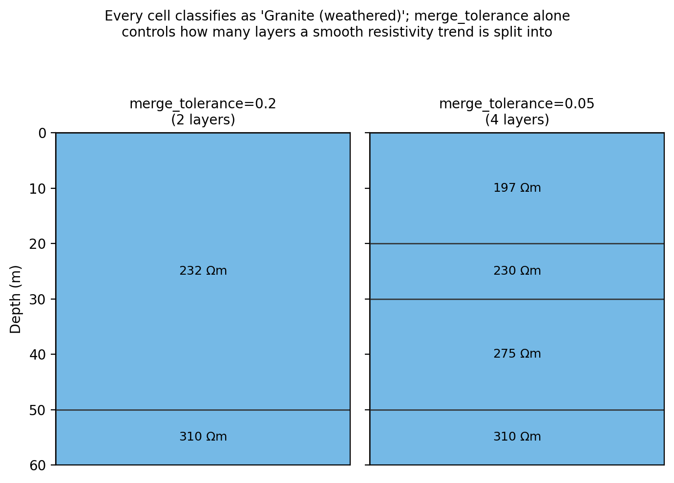
The same six cells, same lithology at every depth, split into 2 layers at
merge_tolerance=0.2 and 4 layers at merge_tolerance=0.05. A looser
tolerance treats the whole smooth trend as one unit; a tighter one turns
inversion-cell-scale resistivity variation into apparent bedding.#
A larger merge_tolerance favours fewer, thicker layers and risks
absorbing a real but subtle boundary into one unit; a smaller value favours
more, thinner layers and risks reporting mesh-scale noise as stratigraphy –
the same trade-off Interpretation workflow describes for the calibrator’s own
merge_tolerance parameter, because both paths call the same
from_column merge loop.
Because the loop only ever extends a run while entries[j].name ==
entries[i].name, every cell absorbed into a layer already shares that
layer’s reported lithology by construction – a run can never mix
classifications and still merge. Layer.confidence is documented as the
fraction of matching cells per layer, but under the current merge rule that
fraction is always \(1.0\); do not read a confidence value less than
one from any log produced by from_column today, in this guide’s fixture
or otherwise.
8.2.7. Next steps#
Continue with:
Interpretation workflow for where classification sits inside calibration, review, and export;
Petrophysical toolkit for the resistivity-to-hydraulic-property toolkit that
EMHydroModelandMonteCarloHydrobuild on;Hydrogeophysical interpretation for quantitative water-table, porosity, and saturation estimation;
Export and reporting for the LAS
codefield and the other exporters that consume aStratigraphicLog.