18.14. Broken Hill: MT Field Data To A 3-D Resistivity Model

Every other tutorial in this section either stops at prepared inversion input (Prepare A ModEM Inversion) or runs a small synthetic or profile-scale case. This one follows a single real magnetotelluric survey all the way through: 21 wideband stations recorded over the world-class Broken Hill Pb-Zn-Ag deposit (New South Wales, Australia), from the raw EDI files, through dimensionality analysis and ModEM input construction, to the published 3-D inversion model of AlQahtani et al. (2026) and its geological interpretation.

The survey, the data, and the model were released open-access with the paper. pyCSAMT bundles a working subset under data/MT/broken-hill; see that folder’s README.md for the exact provenance and the citations you must reproduce if you use the data (repeated under See Also below).

18.14.1. What You Will Learn

After this tutorial you should be able to:

• load a real EDI survey whose station identifiers are unset in the header, and understand why pyCSAMT still keeps the 21 soundings distinct;

• run station_confidence_table() and read the spread of composite confidence across a small wideband survey;

• decide between a 2-D and a 3-D inversion from build_phase_tensor_table() and a multi-frequency phase-tensor map, rather than by assumption;

• build native ModEM 3-D input from the EDIs with InputBuilder;

• load a completed ModEM run with InversionResult, check how well the model fits the data, and render geo-referenced depth maps, a depth-integrated conductance map, and an arbitrary-azimuth vertical section;

• connect those figures back to the paper’s central result – a resistive upper crust hosting discrete shallow conductors on the ore horizon.

18.14.2. Starting Point

The bundled data lives under data/MT/broken-hill:

edis/

21 Phoenix EMpower EDI exports (BH_1 … BH_21), each carrying a full impedance tensor and a vertical-field (tipper) transfer function.

final-models/

The published ModEM inversion: BH_31.dat (the observed data with its real error floors), BH_31_NLCG_030.dat (the model response), BH_31_NLCG_030.res (residuals), and the recovered resistivity model BH_31_NLCG_030.rho (WS format).

Every path below is a plain string. To run this tutorial against your own MT survey, replace data/MT/broken-hill/edis with your EDI directory; the inversion-result section needs a completed ModEM run directory in place of data/MT/broken-hill/final-models.

>>> from pathlib import Path

>>> import matplotlib.pyplot as plt
>>> import numpy as np

>>> run_root = Path("runs/broken_hill")
>>> run_root.mkdir(parents=True, exist_ok=True)
>>> figure_dir = run_root / "figures"
>>> figure_dir.mkdir(exist_ok=True)

18.14.3. Loading The Survey

pycsamt.api.read_edis() reads the directory into a survey object whose .collection is the station container the rest of the workflow uses.

>>> from pycsamt.api import read_edis

>>> survey = read_edis(
...     "data/MT/broken-hill/edis",
...     recursive=False,
...     progress=False,
... )
>>> sites = survey.collection
>>> print(len(sites))
21

>>> print(sorted(sites.stations())[:3])
['BH_10_imp_rev', 'BH_11_imp', 'BH_12_imp_rev']

Twenty-one stations, keyed by their file stems. That fallback matters here: EMpower writes a literal DATAID=None into every >HEAD block – the real station name lives only in >INFO and the filename – so a collection keyed on the header identifier alone would collapse all 21 soundings onto a single "None" key. pyCSAMT treats the placeholder as missing and falls back to the filename stem, which is why len(sites) is 21 and not 1.

18.14.4. Station Confidence

station_confidence_table() scores each sounding on the smoothness, coverage, and internal consistency of its transfer functions. The "composite" method blends those into one number in [0, 1]; see Inspect and QC a Survey for the full breakdown.

>>> from pycsamt.emtools.qc import station_confidence_table

>>> confidence = station_confidence_table(sites, method="composite", api=True)
>>> table = confidence.to_pandas(copy=True)
>>> print(table[["station", "confidence", "coverage"]].head(5).to_string(index=False))
      station  confidence  coverage
BH_10_imp_rev    0.856651       1.0
    BH_11_imp    0.739758       0.8
BH_12_imp_rev    0.816676       1.0
BH_13_imp_rev    0.815596       1.0
BH_14_imp_rev    0.812210       1.0

>>> print(round(table["confidence"].min(), 3),
...       round(table["confidence"].median(), 3),
...       round(table["confidence"].max(), 3))
0.627 0.778 0.876

Composite confidence runs from 0.63 to 0.88 with a median of 0.78 – tight for a real survey, and nothing near a rejection threshold. The one station at coverage = 0.8 (BH_11) simply has a shorter usable band than the rest; that is worth noting before meshing but is not a reason to drop the station. All 21 move forward.

Every station also carries geographic coordinates and a real tipper, which is what makes the dimensionality and mapping steps below possible:

>>> from pycsamt.emtools import ensure_sites

>>> S = ensure_sites("data/MT/broken-hill/edis", recursive=False)
>>> n_coord = sum(
...     1 for s in S
...     if s.coords and np.isfinite(s.coords[0]) and np.isfinite(s.coords[1])
... )
>>> print(n_coord, "/", len(S))
21 / 21

>>> lats = np.array([s.coords[0] for s in S])
>>> lons = np.array([s.coords[1] for s in S])
>>> print(round(float(np.ptp(lats)), 3), round(float(np.ptp(lons)), 3))
0.178 0.187

The survey spans about 0.18 degrees in each direction – roughly 20 km north-south by 18 km east-west at this latitude – an areal deployment, not a single line. That geometry is the first argument for a 3-D inversion; the phase tensor is the second.

18.14.5. Is The Response 2-D Or 3-D?

A 2-D inversion assumes the subsurface can be described by a single geoelectric strike, with no along-strike variation. The phase tensor tests that assumption directly: its skew angle \(\beta\) is a rotationally invariant measure of three-dimensionality that is immune to galvanic static shift, and \(|\beta| \gtrsim 3^\circ\) is the conventional threshold for calling a response 3-D.

>>> from pycsamt.emtools import build_phase_tensor_table

>>> df = build_phase_tensor_table(S)
>>> print(len(df), df["station"].nunique())
1953 21

>>> band = (df["period"] >= 1 / 1000) & (df["period"] <= 1 / 0.008)
>>> frac_3d = (df.loc[band, "skew"].abs() > 3).mean()
>>> print(round(float(frac_3d), 3))
0.397

Across the 0.008-1000 Hz band that the published inversion uses, 40% of all (station, period) cells exceed the 3-degree skew threshold. That is far too much three-dimensionality to justify a 2-D inversion. The plot_phase_tensor_map_grid() view shows where and at what frequency it concentrates:

>>> from pycsamt.emtools import plot_phase_tensor_map_grid

>>> fig = plot_phase_tensor_map_grid(
...     S,
...     frequencies=[30.0, 3.0, 0.3, 0.03],
...     c_by="skew",
...     tipper_convention="parkinson",
...     ellipse_scale=1.3,
...     station_labels="none",
...     ref_ellipse="none",
...     suptitle="Broken Hill -- phase tensor (skew) + Parkinson arrows",
...     recursive=False,
... )
>>> fig.savefig(figure_dir / "phase_tensor_grid.png", dpi=200, bbox_inches="tight")

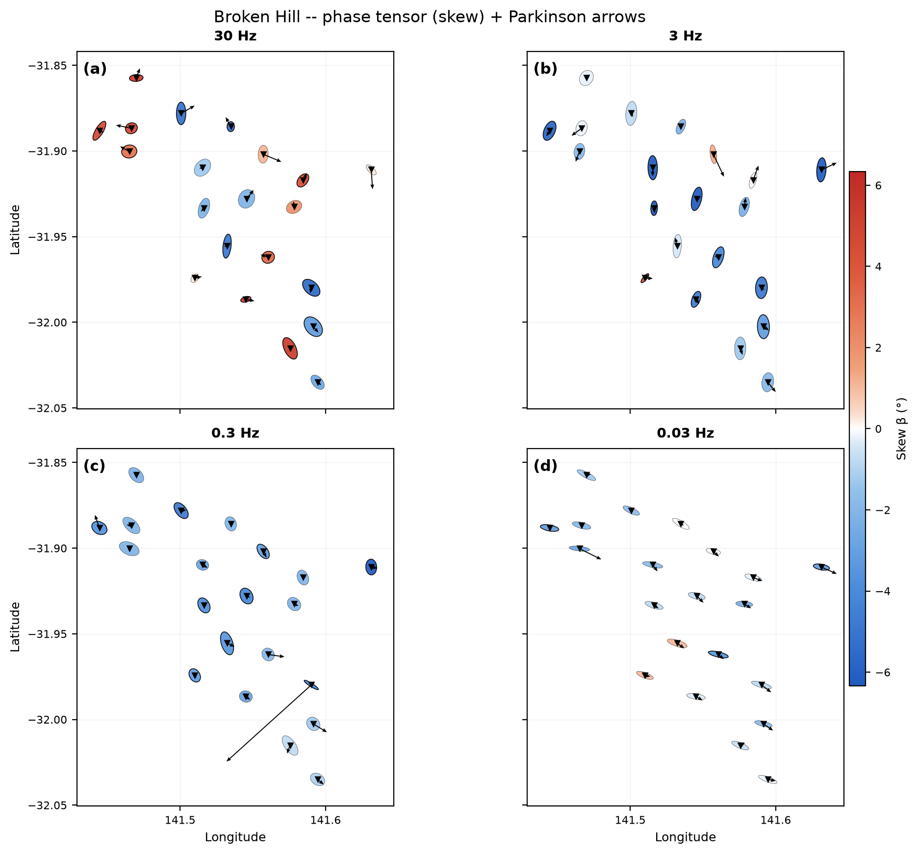
Phase-tensor ellipses filled with skew \(\beta\) (blue negative, red positive) and real induction arrows in the Parkinson convention, at 30, 3, 0.3 and 0.03 Hz.

At 30 Hz – shallowest – the skew is a scatter of blue and red and the ellipses are short and variably oriented: near-surface 3-D structure. By 0.03 Hz almost every ellipse is a similar pale blue and the long axes have aligned NW-SE, so the deep section behaves as a coherent 2-D layer. The induction arrows tell the same story: long at high frequency near the western stations, short and consistent at low frequency. A shallow section broken up by 3-D bodies over a simpler deep section is exactly the case a 2-D inversion cannot represent – and, as it turns out, exactly the geology the paper describes.

18.14.6. Building ModEM 3-D Input

ModEmConfig holds every mesh, error-floor, and inversion-control choice; InputBuilder turns it plus the sites into a native ModEM run directory. The configuration below follows the reasoning in Prepare A ModEM Inversion – a 250 m core cell to match the 2.5 km station spacing, a 50 m first earth layer, a resistive 1000 \(\Omega\cdot\mathrm{m}\) half-space start because the region is known to be resistive, and the full impedance tensor because a 3-D area survey cannot lean on a presumed strike.

>>> from pycsamt.models.modem import ModEmConfig, InputBuilder

>>> cfg = ModEmConfig(
...     mode="3d",
...     component_type="Full_Impedance",
...     error_floor_z=0.05,
...     initial_rho=1000.0,
...     n_airlayers=6,
...     cell_size_h=250.0,
...     cell_size_v_top=50.0,
...     depth_scale=1.1,
...     n_padding_xy=7,
...     nz=45,
...     smooth_x=0.3,
...     smooth_y=0.3,
...     smooth_z=0.3,
...     n_smooth_iter=2,
...     max_iterations=100,
...     target_rms=1.05,
...     binary_3d="Mod3DMT",
... )
>>> workdir = run_root / "modem_input"
>>> written = InputBuilder(config=cfg).build(sites, workdir=workdir)
>>> print(sorted(p.name for p in workdir.iterdir()))
['control.inv', 'covariance.cov', 'data.dat', 'fwd_control.ctrl', 'm0.ws']

>>> from pycsamt.models.modem import ModEmData

>>> built = ModEmData.read(written["data"])
>>> print(built.n_sites, built.n_periods)
21 100

The builder keeps every frequency present in the EDI files – 100 of them here. A production run would decimate to roughly 7 per decade first (Prepare an Occam2D Inversion shows FrequencyFilter doing exactly that); the published Broken Hill run used 24 periods over 0.003-333 s. Running Mod3DMT on workdir is an external step covered in Run Classical Inversions: Occam2D, ModEM, and MARE2DEM. The rest of this tutorial picks up from the authors’ completed run.

18.14.7. The Published Inversion

InversionResult scans a run directory and loads whatever it finds – models, observed and predicted data, covariance, control, and log.

>>> from pycsamt.models.modem import InversionResult

>>> result = InversionResult("data/MT/broken-hill/final-models")
>>> print(result.mode, sorted(result.models))
3d ['iter_0030']

>>> model = result.model_final
>>> print(model.shape)
(55, 120, 129)

>>> rho = model.rho_linear
>>> print(tuple(int(v) for v in np.percentile(rho, [2, 50, 98])))
(55, 247, 1858)

The recovered model is a 129 x 120 cell grid, 55 layers deep. Its resistivity runs from about 55 \(\Omega\cdot\mathrm{m}\) at the conductive 2nd percentile to about 1860 \(\Omega\cdot\mathrm{m}\) at the resistive 98th, with a median near 250 – a resistive model with a conductive tail, the numeric signature of “mostly resistive crust with a few discrete conductors”.

Before interpreting the model, check that it actually fits the data. PlotMisfitMap computes the normalised root-mean-square misfit per station and overall.

>>> from pycsamt.models.modem.plot import PlotMisfitMap

>>> fig = PlotMisfitMap(
...     result=result,
...     use_lonlat=False,
...     show_line_labels=False,
... ).plot()
>>> fig.savefig(figure_dir / "misfit_map.png", dpi=200, bbox_inches="tight")

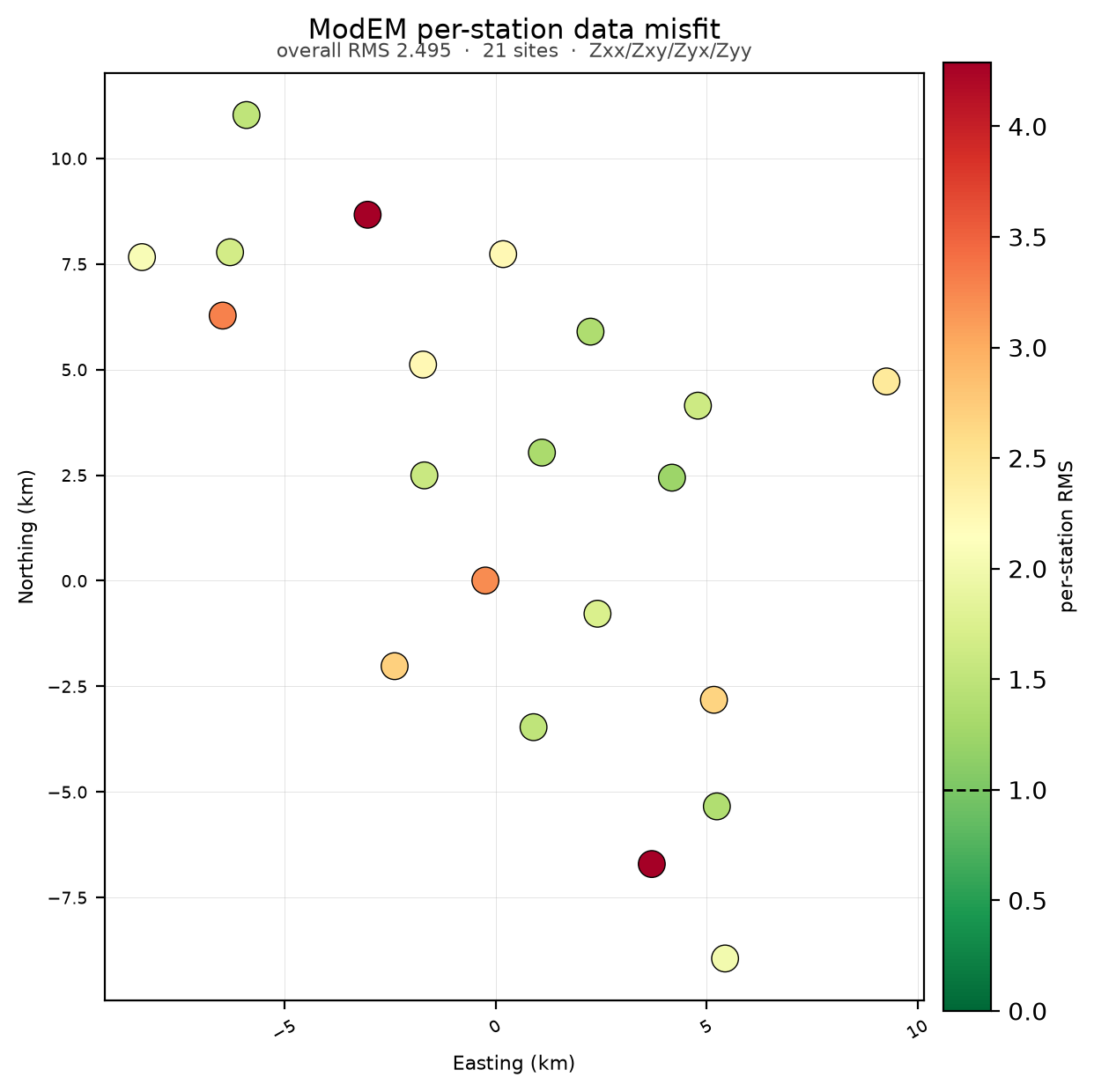
Per-station impedance misfit for the published model. The subtitle reports the overall RMS.

The overall impedance RMS is about 2.5, and most stations sit between 1.5 and 2.5 (green to pale yellow). Two stations reach RMS ~4 (dark red). That is a real, honestly-not-converged inversion: RMS 2.5 is well above the ideal target of 1.0, so absolute resistivity values and sharp boundaries carry less weight than the broad-scale contrast between resistive and conductive domains. No ModEM .log ships with the published model, so the iteration-by-iteration RMS history is not available; result.final_rms is nan for that reason.

18.14.8. Geo-Referenced Depth Maps

PlotDepthMap draws horizontal slices as geographic maps. ModEM data files reduce longitude by 100 degrees (the Broken Hill origin reads 41.53481), so the true value is passed explicitly as origin_lon.

>>> from pycsamt.models.modem.plot import PlotDepthMap

>>> origin = dict(origin_lat=-31.95556, origin_lon=141.53481)
>>> fig = PlotDepthMap(
...     result,
...     depths={"(a) 1 km": 1000, "(b) 2 km": 2000,
...             "(c) 3 km": 3000, "(d) 5 km": 5000},
...     rho_range=(1, 10000),
...     mask_outside_hull=True,
...     contours=[1000],
...     scalebar=True,
...     north_arrow=True,
...     title="Broken Hill ModEM -- resistivity depth slices",
...     **origin,
... ).plot()
>>> fig.savefig(figure_dir / "depth_slices.png", dpi=200, bbox_inches="tight")

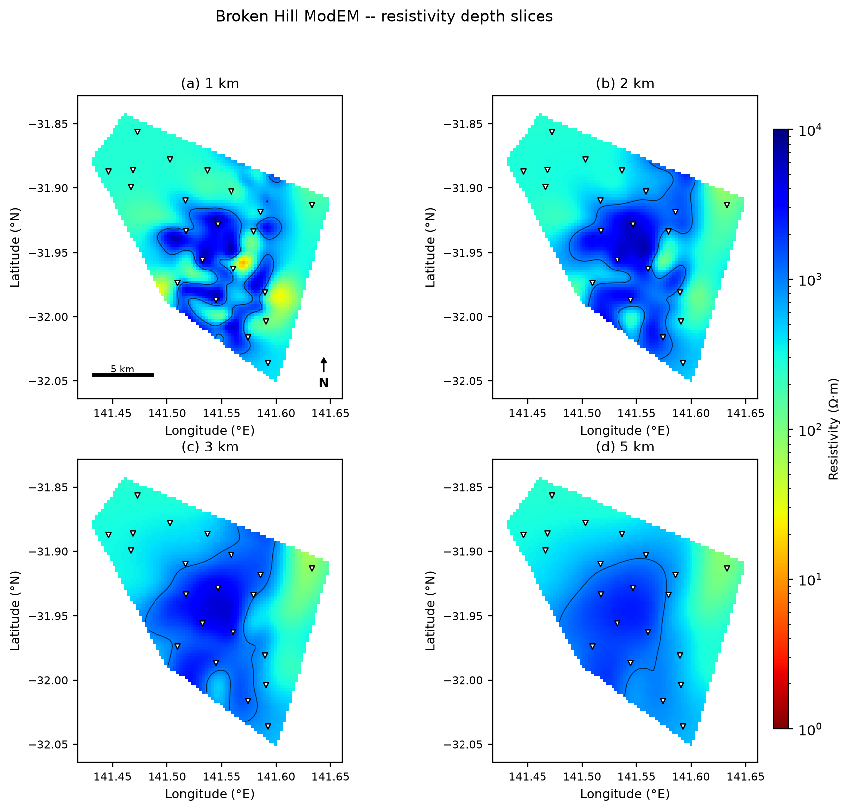
Resistivity at 1, 2, 3 and 5 km. mask_outside_hull=True blanks cells beyond the station convex hull; the black line is the 1000 \(\Omega\cdot\mathrm{m}\) contour.

The crust is resistive everywhere (blue, > 1000 \(\Omega\cdot\mathrm{m}\)), and the resistive core inside the 1000 \(\Omega\cdot\mathrm{m}\) contour grows with depth. At 1 km a handful of small conductive patches (yellow, < 30 \(\Omega\cdot\mathrm{m}\)) sit along the station line in the centre of the survey; by 3 km they have faded. Shallow, discrete, and shrinking downward – consistent with mineralised horizons rather than a deep-rooted conductor.

The most compact single view is a conductance map, the depth integral of conductivity over a window, \(S = \int_{z_1}^{z_2} \sigma \, dz\), in siemens.

>>> fig = PlotDepthMap(
...     result,
...     quantity="conductance",
...     conductance_window=(1000, 6000),
...     render="gouraud",
...     cmap="magma",
...     norm="linear",
...     rho_range=(10, 50),
...     smooth_sigma=0.8,
...     mask_outside_hull=True,
...     station_color="white",
...     cbar_orientation="horizontal",
...     title="Broken Hill -- conductance, 1-6 km",
...     **origin,
... ).plot()
>>> fig.savefig(figure_dir / "conductance.png", dpi=200, bbox_inches="tight")

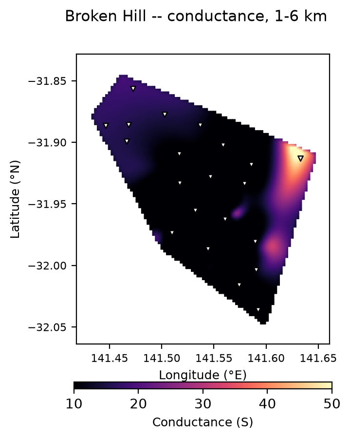
Conductance integrated over 1-6 km. render="gouraud" interpolates between cell centres for the smooth appearance used in published conductance maps.

The interior of the survey is resistive (dark, ~10 S). The conductive anomalies (yellow, up to ~50 S) form an arc along the eastern and south-eastern margin, over the mapped trace of the sulphide-bearing Broken Hill Group. This is the map an MT mineral survey is usually reduced to before it is overlaid on geology and potential-field data.

18.14.9. A Vertical Section

PlotSection in arbitrary-azimuth mode cuts the model along any geographic line. A NW-SE cut runs across the regional structural grain.

>>> from pycsamt.models.modem.plot import PlotSection

>>> fig = PlotSection(
...     result=result,
...     start_point=(-31.860, 141.490),
...     end_point=(-32.020, 141.610),
...     use_latlon=True,
...     origin_lat=-31.95556,
...     origin_lon=141.53481,
...     n_samples=320,
...     depth_max=8000.0,
...     rho_min=1.0,
...     rho_max=5000.0,
...     show_station_names=False,
...     station_tol=2500.0,
...     figsize=(11.5, 4.6),
...     title="Broken Hill ModEM -- section B-B' (NW -> SE)",
... ).plot()
>>> fig.savefig(figure_dir / "section.png", dpi=200, bbox_inches="tight")

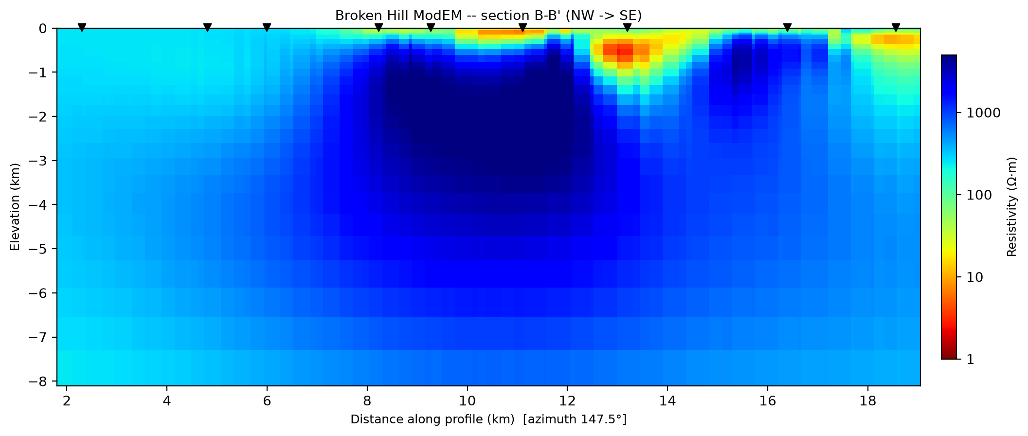
NW-SE section across strike. depth_max=8000 clips the featureless deep model the shallow survey does not constrain.

The section resolves what the depth maps only hint at: the conductors (red/orange, < 10 \(\Omega\cdot\mathrm{m}\)) are discrete bodies confined to the top ~1.5 km of an otherwise uniformly resistive (> 1000 \(\Omega\cdot\mathrm{m}\)) crust. There is no conductive pathway connecting them downward. Because the section is defined by latitude and longitude it can be drawn along the exact trace of a mapped geological cross-section for a one-to-one comparison – which is how the paper ties each conductor to a specific unit of the Broken Hill Group.

18.14.10. What The Model Means

Read together, the figures reproduce the paper’s central observation. The Broken Hill mineral system – one of the largest lead-zinc-silver deposits ever found – sits in a predominantly resistive upper crust. The only conductive anomalies are small, shallow (< 3 km), and spatially tied to the sulphide-rich Broken Hill Group, chiefly the Hores Gneiss. Crucially, none of them connects downward to a lower-crustal conductor.

That matters for exploration. The prevailing “source-to-sink” model expects a major ore system to be underlain by a steep, crustal-scale conductive pathway that once carried metal-bearing fluids. Broken Hill does not preserve one: the authors argue it was severed during granulite-facies metamorphism and later orogeny, leaving only the shallow mineralised horizons behind. Had the deposit’s geology been hidden under sedimentary cover, an exploration program that chased large conductors would have walked straight past it. A resistive MT signature is not, on its own, evidence of a barren crust.

18.14.11. Reusing This With Your Own Data

1. Point read_edis() at your EDI directory. Check len(sites) against the file count – if it collapses, your EDIs likely share a placeholder DATAID, which pyCSAMT already works around by station filename.

2. Run station_confidence_table() and look at the low-confidence tail before meshing.

3. Use build_phase_tensor_table() and plot_phase_tensor_map_grid() to choose 2-D or 3-D. High skew over a meaningful frequency range, or an areal station layout, both point to 3-D.

4. Build input with InputBuilder, decimate the frequency band, and run Mod3DMT externally (Run Classical Inversions: Occam2D, ModEM, and MARE2DEM).

5. Load the finished run with InversionResult, check PlotMisfitMap first, and only then interpret PlotDepthMap and PlotSection.

18.14.12. See Also

Prepare A ModEM Inversion

The full ModEmConfig/InputBuilder walkthrough, including how each mesh and error-floor number is justified from the data.

Run Classical Inversions: Occam2D, ModEM, and MARE2DEM

Compiling and running Mod3DMT (and Occam2D, MARE2DEM), and why most environments should treat the run step as a dry run.

Phase Tensor And Impedance Tensor Tools

The phase-tensor toolkit in depth, including plot_phase_tensor_map_grid.

ModEM

The ModEM integration layer, PlotDepthMap, and PlotSection.

data/MT/broken-hill/README.md

Full data provenance, the survey characteristics, and the required citations.

If you use the Broken Hill data or model, cite both the article and the data release, given in full below.

Data and model citation

AlQahtani, Y., Ozaydin, S., Chatzaras, V., Rey, P. F., & Passos, T. (2026). Why does the Broken Hill deposit sit in resistive crust? Magnetotelluric evidence for metamorphic decoupling of a world-class mineral system. Journal of Geophysical Research: Solid Earth, 131, e2026JB035666. https://doi.org/10.1029/2026JB035666

AlQahtani, Y., Ozaydin, S., Chatzaras, V., Rey, P. F., & Passos, T. (2026). Open data for the article “Why does the Broken Hill deposit sit in resistive crust?”. Zenodo. https://doi.org/10.5281/zenodo.21272106

The survey was acquired by the University of Sydney; the authors acknowledge the Wilyakali/Wiljagali people, Traditional Custodians of the land on which it was recorded. The inversion used ModEM (Kelbert et al., 2014, Computers & Geosciences 66, 40-53).