7.2. Rock resistivity database#

RockDatabase and RockEntry are introduced in Lithology classification, which also covers nearest-midpoint versus overlap classification, the built-in table’s literature provenance, loading a project-specific table from CSV, and the two documented edge cases around non-finite or out-of-range resistivity values – all with a worked example against a real resistivity section, which this page does not repeat. What that page does not cover is where a table can come from besides the bundled default or a CSV file, and what a single RockEntry actually is as an object. Both matter once a project wants to share one table across several tools rather than keep a CSV in sync by hand.

7.2.1. `RockEntry` as a value object#

A RockEntry is a leaf value object in the sense introduced in Package concepts: it never validates rho_min/rho_max against each other, because nothing downstream requires an order between them beyond what its own methods already compute correctly regardless. rho_mid is the geometric-mean midpoint that nearest-midpoint classification searches over, and contains() is the containment check method="overlap" uses:

>>> from pycsamt.geology import RockEntry
>>> entry = RockEntry(
...     name="Laterite", rho_min=80, rho_max=600,
...     color="#B5651D", source="Site report 2024",
... )
>>> entry.rho_mid
219.08902300206645
>>> entry.log_rho_mid
2.340620618687794
>>> entry.contains(150.0), entry.contains(700.0)
(True, False)

A RockDatabase can be built directly from a list of entries, without going through a CSV file at all – useful when entries are generated programmatically rather than typed into a spreadsheet:

>>> from pycsamt.geology import RockDatabase
>>> entries = [
...     entry,
...     RockEntry(name="Saprolite", rho_min=20, rho_max=300,
...               color="#C9A66B", source="Site report 2024"),
...     RockEntry(name="Fresh basement", rho_min=3000, rho_max=200000,
...               color="#4A4A4A", source="Site report 2024"),
... ]
>>> db = RockDatabase(entries)
>>> db
RockDatabase(3 entries)
>>> db.metadata
{}
>>> db.classify(150.0).name
'Laterite'

Note that db.metadata is empty here. Unlike default() (which stamps {"origin": "default"}) or from_csv() (which stamps the source path), the plain constructor does not invent provenance on your behalf – pass metadata= yourself if the table’s origin should travel with it.

Classifying the same three resistivity values against db and against the built-in default makes the point of having more than one table concrete: the query never changes, only the answer does.

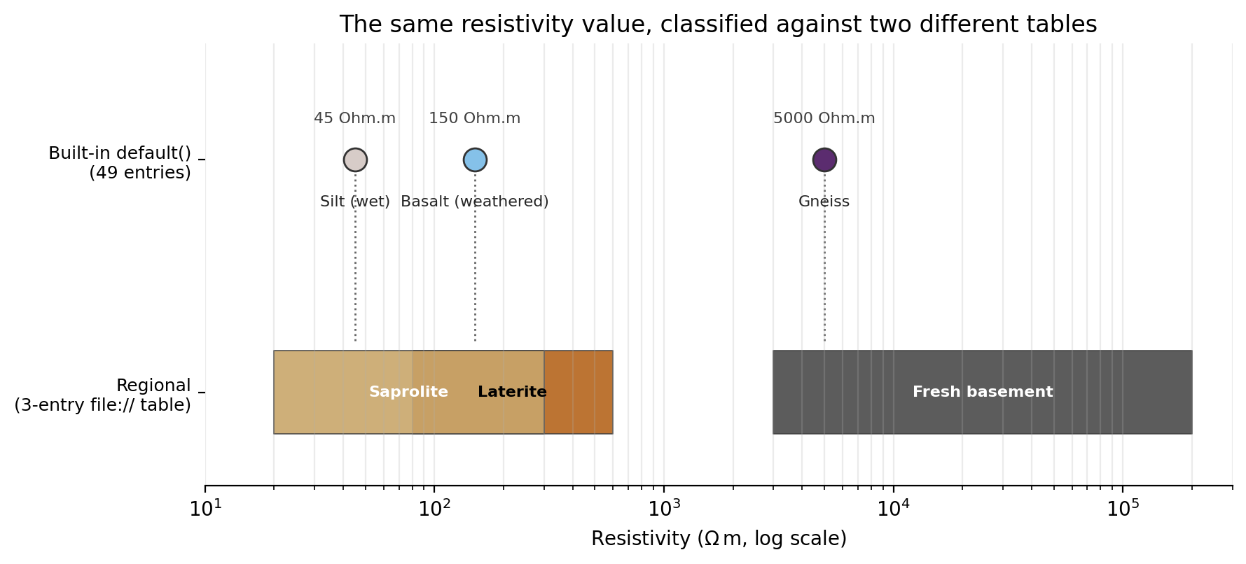
The same three resistivity values classified against the regional table and the built-in default table, with different names each time. — `45`, `150`, and `5000` ohm metres, each classified against the three-entry regional table (bottom) and `RockDatabase.default()` (top, dot color and label only – its full 49-entry range chart is already in Lithology classification). Every one of the three values gets a different name from the two tables; a downstream map or report is only as meaningful as the table it was classified against, which is exactly why that table’s provenance belongs in `metadata`.#

7.2.2. Sourcing a table from elsewhere#

No public, machine-readable service currently maps a rock or lithology name directly to a resistivity range – Data Series 595 covers 90 samples from one watershed, the Geochemical and Geophysical Characteristics of the Conterminous US dataset’s rasters are compressive strength and hydraulic conductivity rather than resistivity, and Macrostrat’s REST API covers lithology names and stratigraphic units rather than resistivity values. That is why BUILTIN_ROCKS is a literature compilation rather than a live fetch. It does not mean a table must always be either that compilation or a hand-maintained CSV, though: a project or organisation with its own controlled table – an internal REST endpoint, a JSON file on a shared drive or object store – can plug it in through RockPropertyProvider, a two-method contract every rock-property source satisfies:

>>> from pycsamt.geology.rock_providers import (
...     RockPropertyProvider, LocalRockPropertyProvider,
... )
>>> isinstance(LocalRockPropertyProvider(), RockPropertyProvider)
True

fetch() returns (entries, metadata) – a list of RockEntry plus a small provenance dictionary – and that is the entire contract; LocalRockPropertyProvider above simply wraps default() or from_csv() behind it, so it can stand in wherever a provider is expected but no remote source is actually involved.

RemoteRockPropertyProvider is the provider behind from_url(): it fetches a JSON array of objects shaped like RockEntry from any URL urllib.request.urlopen() can open, including file:// for a table on a shared drive, not only http(s)://. The example below writes a small regional table to disk and loads it back purely as a local file URL – no network access involved, and the same mechanics apply to an internal https:// endpoint:

>>> import json
>>> from pathlib import Path

>>> table_path = Path("configuration/regional_rocks.json")
>>> table_path.parent.mkdir(parents=True, exist_ok=True)
>>> _ = table_path.write_text(json.dumps([
...     {"name": "Laterite", "rho_min": 80, "rho_max": 600,
...      "color": "#B5651D", "source": "Site report 2024"},
...     {"name": "Saprolite", "rho_min": 20, "rho_max": 300,
...      "color": "#C9A66B", "source": "Site report 2024"},
...     {"name": "Fresh basement", "rho_min": 3000, "rho_max": 200000,
...      "color": "#4A4A4A", "source": "Site report 2024"},
... ]))

>>> db_remote = RockDatabase.from_url(
...     table_path.resolve().as_uri(),
...     cache_dir="configuration/rock_db_cache",
... )
>>> db_remote.classify(150.0).name
'Laterite'
>>> db_remote.metadata["origin"], db_remote.metadata["cache_hit"]
('url', False)

A second call within ttl_seconds (one day by default) reuses the cached response instead of fetching again:

>>> db_remote_again = RockDatabase.from_url(
...     table_path.resolve().as_uri(),
...     cache_dir="configuration/rock_db_cache",
... )
>>> db_remote_again.metadata["cache_hit"]
True

The cache lives under cache_dir (configuration/rock_db_cache above; $PYCSAMT_ROCKDB_CACHE or ~/.pycsamt/rock_db by default), keyed by a hash of the URL, matching the convention already used by pycsamt.ai._zoo’s pretrained-model cache. Pass force=True to bypass a fresh cache entry and re-fetch anyway.

If the fetch itself fails – network error, timeout, or a response that is not a JSON array shaped like RockEntry – from_url does not raise by default. It falls back first to a stale cache entry from an earlier successful fetch, if one exists, and otherwise to LocalRockPropertyProvider, i.e. the same built-in table default() returns:

>>> db_fallback = RockDatabase.from_url(
...     "file:///no/such/table.json",
...     cache_dir="configuration/rock_db_cache",
... )
>>> db_fallback.metadata["origin"]
'default-fallback'
>>> len(db_fallback)
49

Warning

Falling back silently is convenient for a demo but can mask a genuinely broken endpoint in production – a database quietly swapping from a regional table to the generic built-in one changes every classification downstream without an obvious signal. Check metadata["origin"] after every from_url()/from_provider() call in an automated pipeline, or pass fallback=False to raise RockProviderFetchError instead and handle the failure explicitly.

from_provider() is the generic entry point behind from_url – call it directly for anything that is not a plain URL fetch, such as a provider pre-configured with authentication, one composing several sources, or a lightweight provider written for a single project. Nothing beyond the two-method protocol is required:

>>> class InMemoryProvider:
...     def __init__(self, entries):
...         self._entries = entries
...     def fetch(self):
...         return list(self._entries), {"origin": "in-memory"}

>>> provider = InMemoryProvider([entry])
>>> isinstance(provider, RockPropertyProvider)
True
>>> db_custom = RockDatabase.from_provider(provider)
>>> db_custom, db_custom.metadata
(RockDatabase(1 entries), {'origin': 'in-memory'})

7.2.3. Where to go next#

Lithology classification covers classification itself in depth – nearest-midpoint versus overlap matching, extrapolation beyond the table’s coverage, and classifying a full resistivity section. Borehole logs and Structural measurements cover the other two data families in this package.

7.2. Rock resistivity database#

7.2.1. RockEntry as a value object#

7.2.2. Sourcing a table from elsewhere#

7.2.3. Where to go next#

7.2.1. `RockEntry` as a value object#