
5.5. One-Call Topography-Embedded Sections#
The previous three pages built a terrain-embedded figure by hand:
extract_chainage()/
extract_elevation() to read the terrain,
drape_section() to warp the grid, and
draw_topo_section()/
draw_topo_strip() to draw the result, in
that order, with axes limits set before the overlay call.
pycsamt.topo.section is that exact pipeline collapsed into one
call. build_topo_section() runs it and
returns the resolved arrays as a
TopoSection;
plot_topo_section() does the same and
renders the figure. What makes this page substantial rather than a
thin wrapper is everything before the pipeline starts: a model
adapter layer that accepts most of the result types pyCSAMT produces,
and a topography resolver that accepts several different sources and
has to pick one when more than one is available.
5.5.1. Any model, one grid#
Internally, build_topo_section() calls a
private adapter that inspects whatever model it was given and
converts it to a common (x_centers, z_centers, rho_log10) form,
trying each of the following in order until one matches. A plain
tuple is the simplest case – centre positions and a value in
\(\log_{10}(\Omega\cdot\mathrm{m})\) – and needs no conversion at
all:
>>> x_c = np.linspace(0, 2400, 24)
>>> z_c = np.linspace(20, 1500, 30)
>>> rho = np.random.default_rng(2).random((30, 24)) * 2.5 + 0.5

>>> from pycsamt.topo import build_topo_section
>>> sec = build_topo_section((x_c, z_c, rho), elevation=np.full(24, 90.0), chainage=x_c / 1000.0)
>>> sec.method
'array'
A pycsamt.interp.ResistivityModel – the package’s
method-agnostic 2-D container, already in the same
centres/log10(rho) convention – passes straight through, carrying
its own method tag and RMS along with it:
>>> from pycsamt.interp import ResistivityModel
>>> rm = ResistivityModel.from_array(rho, x_c, z_c, method="occam2d", rms=1.42)
>>> sec = build_topo_section(rm, elevation=np.full(24, 90.0), chainage=x_c / 1000.0)
>>> sec.method, sec.rms
('occam2d', 1.42)
A backend-neutral pycsamt.inversion.results.InversionResult
is not itself in that form, but it knows how to get there –
build_topo_section calls its own
result.to_resistivity_model() and continues from the
ResistivityModel it returns, then labels the
result with the result’s backend and method rather than the generic
"occam2d"/"generic" tag ResistivityModel would carry on
its own:
>>> from pycsamt.inversion.results import InversionResult
>>> ir = InversionResult(
...     method="mt", dimension="2d", backend="simpeg", rms=0.91,
...     model={"rho_2d": rho, "x_centers": x_c, "z_centers": z_c},
... )
>>> sec = build_topo_section(ir, elevation=np.full(24, 90.0), chainage=x_c / 1000.0)
>>> sec.method, sec.rms
('simpeg:mt', 0.91)
Two more forms are recognised by shape rather than by type, which
matters for anyone holding a native backend result rather than one
already wrapped in pyCSAMT’s own classes. A native
pycsamt.models.occam2d.results.InversionResult is detected by
the presence of .rho_2d and .mesh – attributes any object with
that shape carries, not only the real class – and is converted with
from_occam2d():
>>> def cell_edges(c):
...     e = np.empty(c.size + 1)
...     e[1:-1] = 0.5 * (c[:-1] + c[1:])
...     e[0] = c[0] - (e[1] - c[0])
...     e[-1] = c[-1] + (c[-1] - e[-2])
...     return e

>>> class _FakeMesh:
...     def __init__(self, x_nodes, z_nodes):
...         self.x_nodes, self.z_nodes = x_nodes, z_nodes
>>> class _FakeOccamData:
...     def __init__(self, offsets, sites):
...         self.offsets, self.sites = offsets, sites
>>> class _FakeOccam2DResult:
...     def __init__(self, rho_2d, x_nodes, z_nodes, station_names, final_rms):
...         self.rho_2d = rho_2d
...         self.mesh = _FakeMesh(x_nodes, z_nodes)
...         self.data = _FakeOccamData(0.5 * (x_nodes[:-1] + x_nodes[1:]), station_names)
...         self.final_rms = final_rms

>>> fake_occam = _FakeOccam2DResult(
...     rho, cell_edges(x_c), cell_edges(z_c),
...     [f"O{i:02d}" for i in range(24)], final_rms=1.68,
... )
>>> sec = build_topo_section(fake_occam, elevation=np.full(24, 90.0), chainage=x_c / 1000.0)
>>> sec.method, sec.rms
('occam2d', 1.68)
A native 2-D pycsamt.models.modem.results.InversionResult is
detected the same way, by a .mode attribute plus a
.model_final/.model_initial object exposing .x_widths,
.z_widths, and .rho_loge (ModEM’s natural-log convention,
divided by \(\ln 10\) on the way in):
>>> class _FakeModEmModel2D:
...     def __init__(self, x_widths, z_widths, rho_loge):
...         self.x_widths, self.z_widths, self.rho_loge = x_widths, z_widths, rho_loge
>>> class _FakeModEmResult:
...     def __init__(self, mode, model_final):
...         self.mode, self.model_final, self.model_initial = mode, model_final, None

>>> x_widths, z_widths = np.diff(cell_edges(x_c)), np.diff(cell_edges(z_c))
>>> fake_modem_2d = _FakeModEmResult("2d", _FakeModEmModel2D(x_widths, z_widths, np.log(10.0 ** rho)))
>>> sec = build_topo_section(fake_modem_2d, elevation=np.full(24, 90.0), chainage=x_c / 1000.0)
>>> sec.method
'modem'
A native 3-D ModEM result is deliberately rejected rather than guessed at – a full volume has no single profile to draw without first choosing a cut, which is a decision this function should not make silently:
>>> fake_modem_3d = _FakeModEmResult("3d", _FakeModEmModel2D(x_widths, z_widths, np.log(10.0 ** rho)))
>>> try:
...     build_topo_section(fake_modem_3d)
... except ValueError as exc:
...     print(exc)
Native 3-D ModEM InversionResult objects hold a full volume, not a single profile. Extract a 2-D cut first (e.g. pycsamt.models.modem.section.station_curtain or pycsamt.models.modem.plot.PlotSection) and pass the resulting (x_centers, z_centers, rho_2d) grid, or a pycsamt.interp.ResistivityModel.
The last recognised form is an AI agent-style result – a plain
dict or an AgentResult, both of
which answer "pred_rho" in obj and obj.get(...) the same way –
exposing pred_rho shaped (n_stations, n_layers) in
\(\log_{10}\rho\), the transpose of every other adapter’s
convention, so it is transposed back on the way in. Its depths_km
are trusted as already being kilometres, unconditionally:
>>> ai_result = {
...     "pred_rho": rho.T,
...     "depths_km": z_c / 1000.0,
...     "station_names": [f"AI{i:02d}" for i in range(24)],
...     "rms_global": 0.74,
... }
>>> sec = build_topo_section(ai_result, elevation=np.full(24, 90.0), chainage=x_c / 1000.0, model_unit="km")
>>> sec.method, sec.rms, sec.values.shape
('ai', 0.74, (30, 24))
Everything else raises rather than guessing. A native MARE2DEM result
uses an unstructured triangular mesh with no (x_centers, z_centers)
grid to fall back to, so it gets a specific, actionable
NotImplementedError instead of a silent misinterpretation, and any
truly unrecognised type gets a TypeError listing what is
accepted:
>>> class _FakeMare:
...     pass
>>> _FakeMare.__module__ = "pycsamt.models.mare2dem.mesh"
>>> try:
...     build_topo_section(_FakeMare())
... except NotImplementedError as exc:
...     print(str(exc)[:88])
Native MARE2DEM results use an unstructured triangular mesh and are not natively support

>>> try:
...     build_topo_section(object())
... except TypeError as exc:
...     print(str(exc)[:66])
Unsupported model type: <class 'object'>. Expected a (x_centers, z
5.5.2. Resolving topography#
With a grid in hand, build_topo_section still needs an elevation
profile, and topo_source="auto" (the default) checks three
possibilities in a fixed order: sites first, then an explicit
elevation array, then terrain inferred directly from the model’s
own air-like cells – the same air-cell logic Draping Flat Grids Over Terrain covered for
mask_above_topo(), reused here to find a
terrain profile rather than to mask cells above one. Giving it a grid
with a real, laterally-varying air cap recovers relief that was never
explicitly supplied as elevation data at all:
>>> flat_x, flat_z = np.linspace(0, 5, 10), np.linspace(0.05, 2.0, 20)
>>> flat_rho = np.random.default_rng(0).random((20, 10)) * 3.0
>>> flat_rho[:2, :] = 6.0     # every column: a 2-row air cap
>>> flat_rho[2:5, 5:] = 6.0   # right half only: 3 more air rows above it

>>> sec = build_topo_section((flat_x, flat_z, flat_rho), topo_source="model")
>>> sec.topo_source
'model'
>>> np.round(sec.elev_km, 4)
array([-0.0003, -0.0003, -0.0003, -0.0003, -0.0003, -0.0006, -0.0006,
       -0.0006, -0.0006, -0.0006])
The right half, with its thicker air cap, comes out at a lower
inferred elevation than the left – more air between a fixed model top
and the first earth cell means the ground itself sits further down.
This is deliberately a relative profile with no absolute datum (the
model top is treated as elevation zero), which is why "sites" and
"array" both take priority over it in "auto" mode whenever a
real, absolute elevation source is available. When none of the three
resolves – no sites, no elevation, and no detectable air cap
– the result is a flat datum and a UserWarning, exactly as
extract_elevation() warns on an all-zero
array in Extracting Station Topography:
>>> import warnings
>>> with warnings.catch_warnings(record=True) as caught:
...     warnings.simplefilter("always")
...     sec = build_topo_section((flat_x, flat_z, np.random.default_rng(1).random((20, 10)) * 3.0))
>>> sec.topo_source
'flat'
>>> "flat datum" in str(caught[0].message)
True
5.5.3. Depth window and units – a real gotcha#
depth_min/depth_max and the model’s own coordinates share one
unit knob, model_unit (default "m"), except for AI-style
results, whose depths_km are always treated as kilometres
regardless of what model_unit says. That exception is easy to
forget, and forgetting it does not raise an error – it silently
produces the full depth range instead of the crop that was asked for:
>>> ai_km_result = {"pred_rho": rho.T, "depths_km": z_c / 1000.0,
...                  "station_names": [f"S{i:02d}" for i in range(24)]}
>>> with warnings.catch_warnings(record=True) as caught:
...     warnings.simplefilter("always")
...     sec_wrong = build_topo_section(
...         ai_km_result, elevation=np.full(24, 90.0), chainage=x_c / 1000.0,
...         depth_max=1.0,  # intended as 1.0 km
...     )
>>> sec_wrong.depth_max_km  # got the full range instead of 1.0 km
1.5
>>> "selects no layers" in str(caught[0].message)
True

>>> sec_right = build_topo_section(
...     ai_km_result, elevation=np.full(24, 90.0), chainage=x_c / 1000.0,
...     depth_max=1.0, model_unit="km",
... )
>>> sec_right.depth_max_km
0.9896551724137932
Left at the default model_unit="m", depth_max=1.0 was read as
1.0 metre – 0.001 km – which selects no layers at all in a grid
whose shallowest cell is already at 20 m, so build_topo_section
falls back to the full range and only a UserWarning marks that
anything unusual happened. Setting model_unit="km" to match the AI
result’s own depths_km convention makes depth_max=1.0 mean
what it looks like it means. The rule to keep straight: model_unit
governs every array-based model’s coordinates and both depth bounds
together, and AI-style results need it set to "km" explicitly to
keep depth cropping meaningful.
5.5.4. Colour scaling ignores outliers by default#
plot_topo_section picks vmin/vmax from the 2nd and 98th
percentile of the visible values, not their raw minimum and maximum,
so one extreme cell does not wash out the rest of the section into a
single colour:
>>> from pycsamt.topo import plot_topo_section

>>> outlier_x, outlier_z = np.linspace(0, 5, 12), np.linspace(0.02, 1.5, 24)
>>> outlier_rho = np.random.default_rng(7).random((24, 12)) * 3.0
>>> outlier_rho[0, 0] = 10.0  # far outside the rest of the section

>>> ax, data = plot_topo_section(
...     (outlier_x, outlier_z, outlier_rho), elevation=np.full(12, 100.0),
...     chainage=outlier_x, model_unit="km", return_data=True,
... )
>>> data.values.max()
10.0
>>> ax.collections[0].get_clim()
(0.06255543408323276, 2.9063956259284156)
The cell is still there – data.values.max() is still 10.0 –
but the colour axis clips at roughly the 2nd/98th percentile of the
whole grid, so the outlier renders as flat, saturated colour instead
of compressing every other cell’s contrast toward the middle of the
colourmap. Passing explicit vmin/vmax bypasses this entirely
when a fixed, comparable scale across several figures matters more
than adapting to any one section’s own outliers.
5.5.5. Default styling: white air, white markers#
draw_topo_section’s own default, covered in Terrain Overlays on Section Axes, tints
the space above the terrain with TopoConfig.fill_color and draws
station pins in whatever colour
pycsamt.api.station.PYCSAMT_STATION_RENDERING happens to be
configured with globally – reasonable defaults for a standalone
terrain overlay, but not necessarily for a filled resistivity
section, where a tinted “sky” competes visually with the colourmap
and a solid marker can disappear into a dark cell of the same section.
plot_topo_section overrides both, deliberately, rather than
inheriting them unchanged:
>>> ax, data = plot_topo_section(
...     (x_c, z_c, rho), elevation=np.full(24, 90.0), chainage=x_c / 1000.0,
...     return_data=True,
... )
>>> scatter = ax.collections[-1]  # the station-pin PathCollection
>>> scatter.get_facecolor(), scatter.get_edgecolor()
(array([[1., 1., 1., 1.]]), array([[0., 0., 0., 1.]]))
>>> [p.get_alpha() for p in ax.patches]  # the above-surface fill polygon
[0.0]
the above-surface fill is switched off (
fill_alpha=0.0) by building its own defaultTopoConfigrather than reusingPYCSAMT_TOPO, so the air stays plain white and any leftover mismatched-column gap (Terrain-Following Coordinates) blends into it instead of standing out as a separately-coloured patch;station markers default to a white face with a black edge – a
StationMarkerStylebuilt once insideplot_topo_section, copied from the globalinversionpreset’s size/linewidth/zorder but withfacecolor="white"– which stays legible sitting on top of any colour incmap, including the dark end of"jet_r"a solid black marker can vanish into.
Both are overridable: pass topo_cfg= for full control over the
terrain fill/line styling, or station_marker= with an explicit
StationMarkerStyle to change only the
markers – for example, to match a project’s existing black-marker
convention rather than this function’s default.
5.5.6. Terrain-draped section, one call#
Putting a full example together – a synthetic
ResistivityModel built on the real L18PLT
station positions, with a conductive body centred beneath the
profile – shows the default kind="pcolormesh" render against real
terrain and real station spacing:
>>> x_c = chain_km * 1000.0  # metres, one column per station
>>> z_c = np.geomspace(15, 1200, 26)  # metres
>>> Xc, Zc = np.meshgrid(x_c, z_c)
>>> body_rho = (
...     2.2
...     - 0.9 * np.exp(-((Zc - 400.0) ** 2) / (2 * 250.0 ** 2))
...     - 0.5 * np.exp(-((Xc - 1600.0) ** 2) / (2 * 500.0 ** 2))
... )
>>> rm = ResistivityModel.from_array(
...     body_rho, x_c, z_c, station_x=x_c, station_names=names,
...     method="occam2d", rms=1.31,
... )

>>> fig, ax = plt.subplots(figsize=(10.5, 5.2))
>>> _ = plot_topo_section(rm, sites=sites, ax=ax, kind="pcolormesh",
...                        vmin=0.6, vmax=2.2, colorbar=True)
>>> fig.savefig("section_two_kinds.png", dpi=170, bbox_inches="tight")
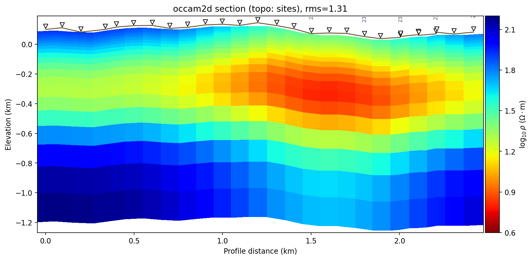
The conductive body visibly follows the terrain the way
Terrain-Following Coordinates first showed, the sky stays plain white above the
terrain line, and the white-faced markers read clearly against both
the pale-blue background and the darker conductive body. A single
wide panel gives the terrain line and station markers room to
breathe, which is why this is the kind this guide leads with;
plot_topo_section() also accepts
kind="imshow" for a flat pseudosection with a separate elevation
strip, but that path is less mature and not covered further here.#
The example above is exactly the point of collapsing Extracting Station Topography,
Draping Flat Grids Over Terrain, and Terrain Overlays on Section Axes into one call: the earlier pages’
manual pipeline still runs underneath, in the same order, but a caller
only has to decide what to plot, not re-derive axes-limit ordering or
pick between drape_section and a flat imshow by hand every
time. From here, Inversion and
AI inversion cover the result objects this page’s
adapters consume in more scientific depth – what an RMS value or a
recovered model actually means – while this page’s job was narrower:
getting any of them onto a page, over real terrain, correctly.