3. Transformers

Every acquisition system ends up writing its own transfer-function file format, and every one of those formats eventually needs to become an EDI so the rest of pyCSAMT – QC, static shift, dimensionality, inversion prep – can treat it the same way. pycsamt.transformers is where that convergence happens: a AVG file, a J-file, a raw cross-power-spectra EDI, or a field time series all enter through a different reader, but each one leaves through the same door, an EDIFile or an EDICollection. A fifth converter, pycsamt.tdem.transform.TEMtoEDI, lives in a different subpackage because its input physics (a transient decay, not a continuous-wave transfer function) is genuinely different, but it honours the exact same contract and is covered here alongside the other four.

3.1. The Transformer Contract

Every converter in this module is a small subclass of TransformerMixin, and every subclass moves data through the same neutral payload, TFBundle. A bundle just holds frequency-indexed arrays – freq, z/z_err, tipper/tipper_err, rho/phase – plus a station name and optional coordinates. Concrete transformers only have to implement two steps: extract (parse the foreign format into a bundle) and emit_edi (build an EDIFile from a finalized one). Everything in between is handled once, by the mixin’s _finalize:

1. resolve a valid station identity, synthesizing one from the station id if the source did not provide a usable name;

2. order frequencies ascending or descending;

3. drop nearly-duplicate frequencies within a relative tolerance;

4. optionally fill z from (rho, phase) or vice versa, if the concrete transformer implements the physics for it.

All four of those steps read from one live settings object, pycsamt.core.config.CoreConfig, so the same policy applies everywhere a bundle is finalized rather than being repeated per format:

>>> from pycsamt.core.config import get_config, config_context
>>> from pycsamt.core.base import TFBundle, ensure_station
>>> import numpy as np
>>> cfg = get_config()
>>> print(cfg.freq_order, cfg.freq_tol, cfg.compute_res_from_z, cfg.compute_z_from_res)
desc 1e-09 True True
>>> raw = TFBundle(
...     freq=np.array([10.0, 10.0000001, 5.0, 20.0]),
...     rho=np.array([80.0, 80.0, 120.0, 40.0]),
...     phase=np.array([45000.0, 45000.0, 42000.0, 48000.0]),
...     station=None,
...     station_id=17,
... )
>>> print(raw.is_empty())
False
>>> print(ensure_station(raw.station, raw.station_id))
S017

freq_order='desc' and a freq_tol of one part in a billion are the project defaults; compute_res_from_z/compute_z_from_res only take effect when the concrete transformer actually implements compute_res_from_z/compute_z_from_res – on the bare mixin they are no-ops, which is worth seeing directly rather than taking on faith:

>>> from pycsamt.transformers import TransformerMixin
>>> class Echo(TransformerMixin):
...     def extract(self, source):
...         return source
...     def emit_edi(self, bundle):
...         return bundle
...
>>> with config_context(freq_order="asc", freq_tol=1e-6):
...     out = Echo()._finalize(raw, station_id=raw.station_id)
...
>>> print(out.station)
S017
>>> print(out.freq)
[ 5. 10. 20.]
>>> print(out.rho)
[120.  80.  40.]
>>> print(out.z)
None

Three things happened inside that one _finalize call: the synthetic name S017 from the earlier example survived (a mixin without physics does not overwrite a name that already validated), the near-duplicate frequency pair 10.0/10.0000001 collapsed to a single 10.0 under the tightened freq_tol, and reordering to asc moved the surviving three frequencies and their matching rho values together. out.z stays None because Echo never overrode compute_z_from_res – AVGtoEDI is the first converter below that actually does.

3.2. Zonge AVG Conversion

An AVG file stores one instrument-averaged transfer-function record per frequency, and a Zonge line file can bundle many stations into one file. data/avg/K1.AVG is a real 47-station CSAMT line; loading it directly with AVG shows the raw tensor shape before any EDI construction happens:

>>> import numpy as np
>>> from pycsamt.zonge.avg import AVG
>>> from pycsamt.transformers import AVGtoEDI
>>> avg = AVG.from_file("data/avg/K1.AVG")
>>> z, f, st = avg.to_tensor(var="z")
>>> print(z.shape, f.shape, len(st), st.min(), st.max())
(47, 17, 2, 2) (17,) 47 150.0 2450.0

Every station carries 17 frequencies, and st here is not a station name but the line chainage in metres – AVGtoEDI turns that numeric distance into a proper station identity through the same ensure_station machinery shown above:

>>> col = AVGtoEDI().transform(avg)
>>> print(type(col).__name__, len(col))
EDICollection 47
>>> print([ed.station for ed in col][:3], "...", [ed.station for ed in col][-3:])
['S150', 'S200', 'S250'] ... ['S2350', 'S2400', 'S2450']
>>> ed0 = col[0]
>>> print(ed0.station, ed0.Z.freq.shape, ed0.has_tipper)
S150 (17,) False
>>> print(ed0.Z.freq[:5])
[8192. 4096. 2048. 1024.  512.]
>>> print(np.round(ed0.Z.res_xy[:5], 6))
[0.000438 0.001193 0.002921 0.006704 0.006543]
>>> print(np.round(ed0.Z.res_yx[:5], 6))
[0. 0. 0. 0. 0.]

res_yx is exactly zero, not noisy-small: K1 is a scalar CSAMT line with only an Ex-Hy receiver pair, the same single-off-diagonal-component situation already worked through in Field Zones: Near, Transition, And Far Field. The resistivities themselves look tiny for a CSAMT line – a few \(\times 10^{-3}\) rather than tens of ohm-metres – because ed0.Z computes them with the legacy Zonge convention \(\rho_a = 0.2\,|Z|^2/f\) on field-unit impedances, not the SI convention; Impedance Tensor derives and names that ~633257x scale gap (RHO_FACTOR/ZONGE_RHO_FACTOR) in full, and it resurfaces below in the TEM section too.

3.3. Attaching Station Topography

An AVG object on its own has no coordinates – avg.topo is None until a matching Zonge .stn file is attached with add_topography(). K1’s companion file, data/avg/K1.stn, records station easting/northing in UTM zone 49N rather than latitude/longitude, which matters for what AVGtoEDI.post_emit can actually populate:

>>> avg2 = AVG.from_file("data/avg/K1.AVG").add_topography(
...     "data/avg/K1.stn", utm_zone="49N",
... )
>>> print(avg2.topo.frame.head(3))
   station     easting     northing  elevation
0      150  748846.846  2883860.032      574.5
1      200  748893.155  2883840.178      572.3
2      250  748935.809  2883812.363      561.3
>>> col_bare = AVGtoEDI().transform(avg2)
>>> h0 = col_bare[0].get_section("head")
>>> print(col_bare[0].station, h0.lat, h0.long, h0.elev)
S150 0.0 0.0 574.5

Elevation came through because the elevation column already exists, but latitude/longitude stayed at the 0.0 placeholder: post_emit only copies coordinates when it finds columns literally named latitude/longitude (or a small set of aliases), and easting/northing do not qualify. Projecting the frame first with convert_coords() closes that gap:

>>> avg2.topo.convert_coords(to="ll", inplace=True)
>>> print(avg2.topo.frame[["station", "latitude", "longitude"]].head(3))
   station   latitude   longitude
0      150  26.052401  113.487159
1      200  26.052214  113.487617
2      250  26.051955  113.488038
>>> col_topo = AVGtoEDI().transform(avg2)
>>> h0 = col_topo[0].get_section("head")
>>> hN = col_topo[-1].get_section("head")
>>> print(col_topo[0].station, round(h0.lat, 5), round(h0.long, 5), h0.elev)
S150 26.0524 113.48716 574.5
>>> print(col_topo[-1].station, round(hN.lat, 5), round(hN.long, 5), hN.elev)
S2450 26.04033 113.50579 410.0

The line runs about 2.3 km along strike and drops roughly 160 m in elevation from its first to its last station – real relief that a later static-shift or topography-drape step would need to see, which is exactly why attaching the .stn file before conversion (rather than after) is worth making a habit.

With coordinates and all 47 stations in hand, the converted line can be plotted directly – three representative soundings side by side with a full along-line pseudosection, reproducing the figure below byte-for-byte:

import matplotlib.pyplot as plt

picks = ["S150", "S1200", "S2450"]
fig, axes = plt.subplots(1, 2, figsize=(11.0, 4.2))

ax = axes[0]
for name in picks:
    ed = next(e for e in col if e.station == name)
    ax.loglog(ed.Z.freq, ed.Z.res_xy, "o-", ms=4, lw=1.3, label=name)
ax.set(xlabel="Frequency (Hz)", ylabel=r"$\rho_{a,xy}$ (field units)",
       title="K1 line: three stations")
ax.legend(fontsize=8)
ax.grid(True, which="both", alpha=0.3)

rho_grid = np.array([e.Z.res_xy for e in col])
dist = np.array([float(e.station.lstrip("S")) for e in col])
ax2 = axes[1]
pc = ax2.pcolormesh(dist, ed0.Z.freq, np.log10(rho_grid).T,
                     shading="auto", cmap="turbo")
ax2.set_yscale("log")
ax2.invert_yaxis()
ax2.set(xlabel="Station chainage (m)", ylabel="Frequency (Hz)",
        title=r"K1 line: $\log_{10}\rho_{a,xy}$")
fig.colorbar(pc, ax=ax2, label=r"$\log_{10}\rho_a$")
fig.tight_layout()

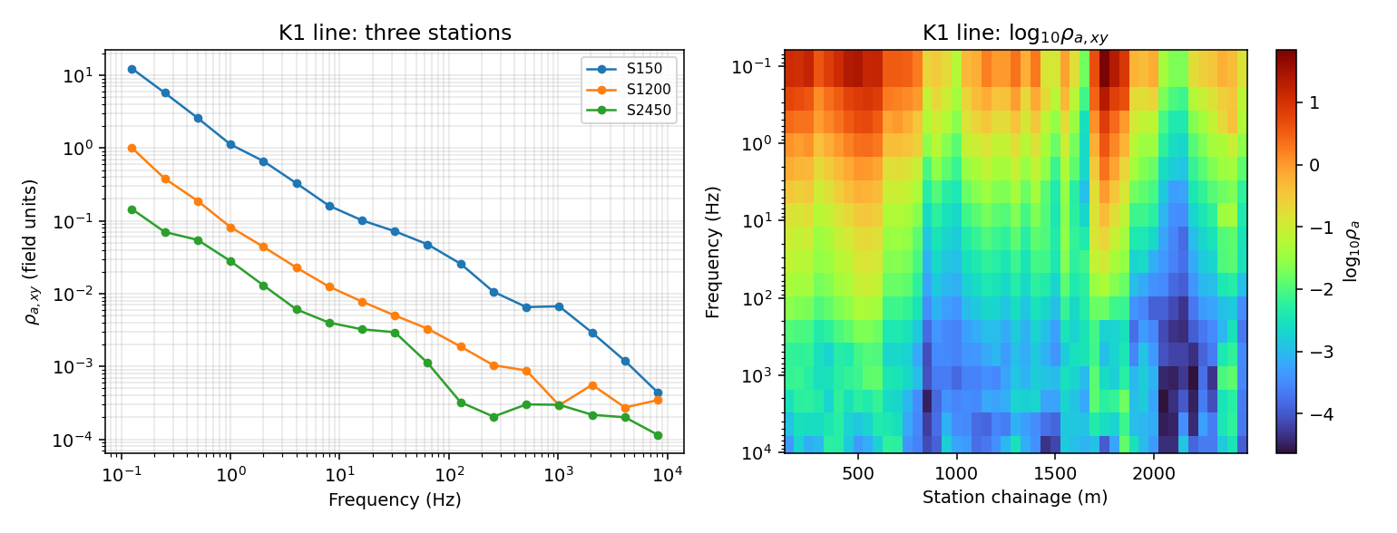
Left: apparent resistivity at three stations spanning the K1 line, all from the same AVGtoEDI().transform(avg) call. Right: the same quantity for every station, showing a resistive zone around station 150-750 m and two conductive zones further along the line.

3.4. Jones J Conversion

A J-file carries the same kind of transfer function as an AVG file, but as a plain-text, one-station-per-file ASCII format from the BIRRP processing lineage. data/j/kb0-s001.txt is a real single-station J-file; JtoEDI accepts either the path or an already-parsed JFile and returns a single EDIFile rather than a collection, because one J-file is one station:

>>> from pycsamt.jones.j import JFile
>>> from pycsamt.transformers import JtoEDI
>>> jf = JFile.from_file("data/j/kb0-s001.txt")
>>> print(jf.station, jf.n_freq, jf.lat, jf.lon, jf.azimuth)
KB0001 29 41.9782 140.8958 330.0
>>> ed_j = JtoEDI().transform(jf)
>>> print(type(ed_j).__name__, ed_j.station, ed_j.Z.freq.shape, ed_j.has_tipper)
EDIFile KB0001 (29,) True
>>> print(ed_j.Z.freq[:6])
[10320.  7020.   270.   256.   192.   128.]
>>> print(np.round(ed_j.Z.res_xy[:6], 6))
[1.39e-04 1.46e-04 7.90e-05 8.60e-05 6.40e-05 4.50e-05]
>>> print(np.round(ed_j.Z.res_yx[:6], 6))
[2.31e-04 2.00e-04 1.56e-04 1.79e-04 8.20e-05 6.80e-05]

Unlike the K1 scalar line, KB0001 has both off-diagonal components populated and a real tipper, so has_tipper is True. The station-naming path is worth a second look here: JFile already carries a valid name (KB0001), so ensure_station keeps it untouched rather than synthesizing one – the same rule demonstrated on the bare mixin earlier now runs for real.

JtoEDI also accepts a whole JCollection and returns an EDICollection in that case, mirroring AVGtoEDI’s multi-station behaviour. data/j/nia holds four J-files that pyCSAMT itself exported from the K1 line – the first station’s coordinates match K1.stn’s 26.0524, 113.48716 exactly, confirming the two directories describe the same physical line in two different formats:

>>> from pycsamt.jones.collection import JCollection
>>> jc = JCollection.from_sources("data/j/nia", recursive=False)
>>> print(len(jc), sorted(jc.stations()))
4 ['NIA000', 'NIA001', 'NIA002', 'NIA003']
>>> col_j = JtoEDI().transform(jc)
>>> print(type(col_j).__name__, len(col_j))
EDICollection 4
>>> print(sorted(ed.station for ed in col_j))
['NIA000', 'NIA001', 'NIA002', 'NIA003']

The single-station conversion above is enough to show what a converted J-file looks like end to end – both off-diagonal apparent-resistivity curves together with their phases, reproducing the figure below:

fig, axes = plt.subplots(1, 2, figsize=(11.0, 4.2))
per = 1.0 / ed_j.Z.freq

ax = axes[0]
ax.loglog(per, ed_j.Z.res_xy, "o-", color="#1f77b4", ms=4, label=r"$\rho_{a,xy}$")
ax.loglog(per, ed_j.Z.res_yx, "s-", color="#d62728", ms=4, label=r"$\rho_{a,yx}$")
ax.set(xlabel="Period (s)", ylabel=r"$\rho_a$ (field units)",
       title=f"J-file conversion ({ed_j.station})")
ax.legend(fontsize=8)
ax.grid(True, which="both", alpha=0.3)

ax2 = axes[1]
ax2.semilogx(per, ed_j.Z.phase_xy, "o-", color="#1f77b4", ms=4, label=r"$\phi_{xy}$")
ax2.semilogx(per, ed_j.Z.phase_yx, "s-", color="#d62728", ms=4, label=r"$\phi_{yx}$")
ax2.set(xlabel="Period (s)", ylabel="Phase (deg)", title="Phase")
ax2.legend(fontsize=8)
ax2.grid(True, alpha=0.3)
fig.tight_layout()

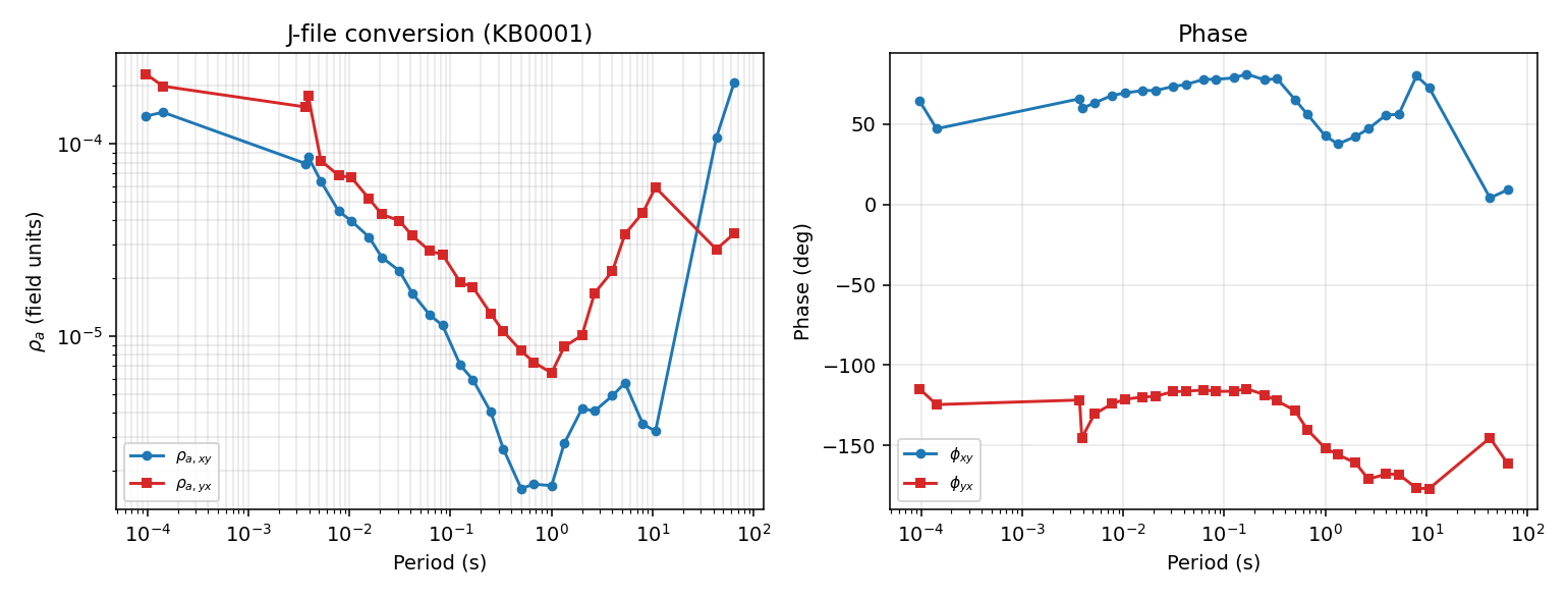
KB0001’s two off-diagonal modes disagree by up to half a decade in resistivity at short period and cross over near 1 s – real 2-D/3-D behaviour rather than the clean antisymmetric pair a 1-D earth would produce.

3.5. Spectra-EDI Conversion

Some instruments export an EDI whose >=SPECTRASECT block holds raw cross-power spectrum estimates instead of a finished impedance tensor – richer, but one processing step short of usable Z. SpectraToEDI closes that last step. For each frequency it forms the electric-magnetic and vertical-magnetic blocks and solves

(1)\[\mathbf{Z}(f) = \mathbf{S}_{EH}(f)\,\mathbf{S}_{HH}^{-1}(f), \qquad \mathbf{T}(f) = \mathbf{S}_{ZH}(f)\,\mathbf{S}_{HH}^{-1}(f),\]

where \(\mathbf{S}_{HH}\) is the magnetic auto-spectral block and \(\mathbf{S}_{EH}\)/\(\mathbf{S}_{ZH}\) are the electric- and vertical-magnetic cross-spectral blocks. data/MT/SPECTRA/spectra01.edi is a de-identified short-period field example with a vertical channel, so both Z and the tipper come out of one call:

>>> from pycsamt.transformers import SpectraToEDI
>>> col_sp = SpectraToEDI(estimate_error=True).transform(
...     "data/MT/SPECTRA/spectra01.edi",
... )
>>> ed_sp = col_sp[0]
>>> print(ed_sp.station, ed_sp.Z.n_freq, ed_sp.has_tipper)
SPECTRA01 51 True
>>> print(ed_sp.Z.freq[:5])
[10400.  8800.  7200.  6000.  5200.]
>>> print(np.round(ed_sp.Z.res_xy[:5], 3))
[119.759  80.02   28.197  20.613  20.13 ]
>>> print(np.round(ed_sp.Tip.amplitude[:5, 0, :], 4))
[[0.2894 0.2028]
 [0.228  0.1531]
 [0.0141 0.0377]
 [0.0152 0.0455]
 [0.0453 0.0325]]

estimate_error=True propagates first-order complex-Wishart impedance uncertainty into the converted EDI’s >ZXX.VAR-style blocks using the degrees of freedom inferred from the spectra file’s own averaging metadata, rather than leaving every error at the config’s error_fill_value.

3.6. Time-Series Conversion

The least processed input this module accepts is a raw field recording: TStoEDI reads Ex/Ey/Hx/Hy samples, builds Hann-tapered overlapping segments, stacks their cross-power spectra with Huber-robust weighting, and solves the same relation as (1) for \(\mathbf{Z}\) – the only difference is that the spectra are estimated here rather than read pre-computed from an EDI block. data/MT/TS/kap103as.ts is a real LiMS time-series recording from the EMSLAB Lincoln Line:

>>> from pycsamt.transformers import TStoEDI
>>> col_ts = TStoEDI(nfft=10240).transform(
...     "data/MT/TS/kap103as.ts/kap103as.ts",
... )
>>> ed_ts = col_ts[0]
>>> print(ed_ts.station, ed_ts.Z.n_freq, ed_ts.has_tipper)
kap103 21 True
>>> print(ed_ts.Z.freq[:5])
[0.05       0.03619604 0.02620306 0.01896894 0.01373201]
>>> print(np.round(ed_ts.Z.res_xy[:5], 3))
[9.12  7.587 6.353 5.242 4.674]

Twenty-one output frequencies from one nfft=10240 FFT segment length is the estimator’s own per-decade frequency choice, not the raw sample count – per_decade controls that resolution directly if a denser or coarser spectrum is wanted.

3.7. One Shape, Two Sources

spectra01.edi and kap103as.ts could not start more differently – one is pre-computed cross-power spectra sitting inside an EDI wrapper, the other is a raw multi-day voltage recording – yet both converters hand back the same EDI-shaped object with the same Z/Tip API. Plotting both conversions together makes that convergence concrete:

fig, axes = plt.subplots(1, 2, figsize=(11.0, 4.2))

ax = axes[0]
per_sp = 1.0 / ed_sp.Z.freq
ax.loglog(per_sp, ed_sp.Z.res_xy, "o-", color="#1f77b4", ms=4, label=r"$\rho_{a,xy}$")
tip_mag = np.hypot(ed_sp.Tip.amplitude[:, 0, 0], ed_sp.Tip.amplitude[:, 0, 1])
ax3 = ax.twinx()
ax3.loglog(per_sp, tip_mag, "^--", color="#2ca02c", ms=4, label="|tipper|")
ax.set(xlabel="Period (s)", ylabel=r"$\rho_{a,xy}$ (field units)",
       title=f"Spectra $\\to$ EDI ({ed_sp.station})")
ax3.set_ylabel("|tipper|", color="#2ca02c")
ax.grid(True, which="both", alpha=0.3)

ax2 = axes[1]
per_ts = 1.0 / ed_ts.Z.freq
ax2.loglog(per_ts, ed_ts.Z.res_xy, "o-", color="#1f77b4", ms=4, label=r"$\rho_{a,xy}$")
ax2.loglog(per_ts, ed_ts.Z.res_yx, "s-", color="#d62728", ms=4, label=r"$\rho_{a,yx}$")
ax2.set(xlabel="Period (s)", ylabel=r"$\rho_a$ (field units)",
        title=f"Time series $\\to$ EDI ({ed_ts.station})")
ax2.legend(fontsize=8)
ax2.grid(True, which="both", alpha=0.3)
fig.tight_layout()

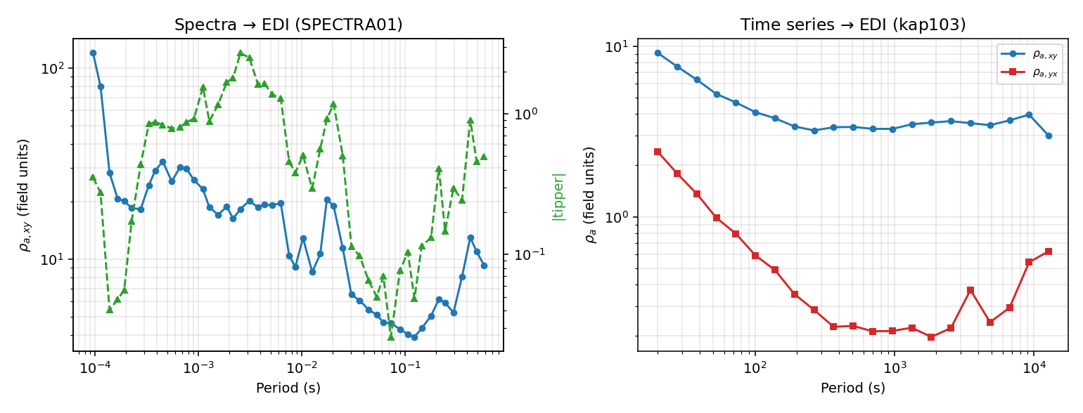
Left: SPECTRA01’s resistivity and tipper magnitude, both already present in the source spectra block. Right: kap103’s two off-diagonal resistivities, estimated here directly from raw voltage samples. Different physics upstream, identical downstream shape.

3.8. TEM Soundings To EDI

pycsamt.tdem.transform.TEMtoEDI closes the same gap for time-domain data: a transient decay has no natural frequency at all, so it first has to be mapped onto a pseudo-frequency axis before it can sit in an EDI’s Z block. The late-time apparent-resistivity formula behind that mapping, the loop-geometry corrections, and the pseudo-frequency convention are worked through in full in TDEM Basics ((4)); this section only covers the conversion contract itself. data/TEMAVG/JIANGSU is a real 2790-sounding TEM survey:

>>> from pycsamt.tdem import read_temavg_soundings, LateTimeTransform, TEMtoEDI
>>> soundings = read_temavg_soundings(
...     "data/TEMAVG/JIANGSU", component="Hz", pattern="*.AVG",
... )
>>> print(len(soundings))
2790
>>> s0 = next(s for s in soundings if s.station_name == "TEM100_100")
>>> print(s0.n_gates, s0.offset, s0.loop_shape, s0.loop_dims, round(s0.moment, 1))
25 0.0 square (360.0,) 1296000.0
>>> lt = LateTimeTransform()
>>> result = lt.transform(s0)
>>> print(result["freq"][:5])
[13.04441792 16.37800929 20.54805282 25.87001887 32.50381764]
>>> print(np.round(result["rho_a"][:5], 2))
[1695.01  879.05  309.75  349.1   334.71]
>>> conv = TEMtoEDI(method="late_time")
>>> col_tem = conv.transform(s0)
>>> ed_tem = col_tem[0]
>>> print(type(col_tem).__name__, len(col_tem))
EDICollection 1
>>> print(ed_tem.station, ed_tem.Z.freq.shape)
TEM100_100 (25,)
>>> print(np.round(ed_tem.Z.res_xy[:5], 2))
[1695.01  879.05  309.75  349.1   334.71]
>>> print(np.round(result["rho_a"][:5] / ed_tem.Z.res_xy[:5], 1))
[1. 1. 1. 1. 1.]

Unlike the K1 line above, there is no scale gap here: ed_tem.Z.res_xy comes back identical to result["rho_a"] (up to floating-point noise). TEMtoEDI builds |Z_xy| as the exact inverse of the legacy Zonge formula EDIFile.Z’s own res_xy property applies when it recomputes resistivity from a packed z – \(|Z_{xy}|=\sqrt{5\,f\,\rho_a}\) – specifically so that this round trip lands back on the same number. Read either result["rho_a"] or ed_tem.Z.res_xy after conversion; they agree, which also means an EDI written from this collection and reopened later will report the same apparent resistivity a caller already trusted from result.

The station’s own decay curve, alongside the apparent resistivity from result, reproduces the figure below:

fig, axes = plt.subplots(1, 2, figsize=(11.0, 4.2))

ax = axes[0]
ax.loglog(s0.time_gates * 1e3, np.abs(s0.dBdt()), "o-",
          color="#1f77b4", ms=4, lw=1.3)
ax.set(xlabel="Time (ms)", ylabel=r"$|\partial B_z/\partial t|$ (T/s)",
       title=f"Decay curve ({s0.station_name})")
ax.grid(True, which="both", alpha=0.3)

ax2 = axes[1]
ax2.loglog(result["freq"], result["rho_a"], "o-", color="#d62728", ms=4, lw=1.3)
ax2.set(xlabel="Pseudo-frequency (Hz)", ylabel=r"$\rho_a$ ($\Omega\cdot$m)",
        title="LateTimeTransform output")
ax2.grid(True, which="both", alpha=0.3)
fig.tight_layout()

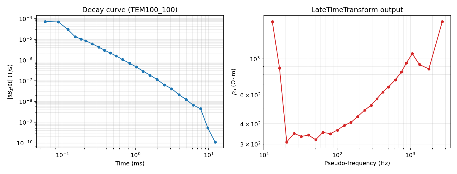
Left: the raw decay, spanning almost five decades before flattening into the noise floor at the latest gates. Right: the transform’s own apparent resistivity, U-shaped rather than a clean sounding – the same honest, unsmoothed result already discussed in TDEM Basics.

3.9. Batch Conversion And Failures

AVGtoEDI and JtoEDI are all-or-nothing: transform raises on the first problem it hits, which is appropriate for a single AVG line or J-file where a broken station usually means the whole file is suspect. SpectraToEDI and TStoEDI process many independent files at once, so they default to skip_errors=True and expose transform_batch(), which always returns a TransformResult instead of raising:

>>> from pathlib import Path
>>> batch_result = SpectraToEDI(skip_errors=True).transform_batch(
...     ["data/MT/SPECTRA/spectra01.edi", "data/CSAMT/csa000.edi"],
... )
>>> print(batch_result)
TransformResult(ok=1, fail=1)
>>> for r in batch_result.failures:
...     print(Path(r.source).name, "->", r.error)
...
csa000.edi -> No >=SPECTRASECT found.
>>> print(sorted(ed.station for ed in batch_result.collection))
['SPECTRA01']

csa000.edi is a perfectly good EDI – it simply carries a finished impedance tensor rather than a raw spectra block, so Spectra correctly refuses it. transform (rather than transform_batch) would raise RuntimeError with the same message the moment skip_errors=False, which is the setting to use once a batch is expected to fully succeed.

3.10. Recording A Workflow Session

Everything above converts one file at a time. pycsamt.session adds two thin layers on top for a whole workflow: a single normalized entry point across source formats, and light, on-disk provenance for whatever a script actually produced.

Normalize dispatches any of the inputs this page has covered – an AVG/JFile object or path, a bare EDIFile, or an existing EDICollection – to the matching transformer and always hands back a collection:

>>> import shutil
>>> from pycsamt.session import Normalize

>>> shutil.rmtree("work/normalize_demo", ignore_errors=True)  # fresh manifest below
>>> with Normalize("work/normalize_demo") as nz:
...     coll = nz.load("data/avg/K1.AVG")
...     same = nz.load(coll)
...
>>> print(type(coll).__name__, len(coll))
EDICollection 47
>>> print(same is coll)
True

An already-normalized EDICollection passes straight through unchanged rather than being re-converted – Normalize is meant to sit at the top of a script where the input format is not known in advance, not to be called defensively before every operation. This is a different normalization from ensure_sites’s own permissive input handling covered in Loading electromagnetic data: Normalize dispatches raw AVG/J/EDI sources to the matching transformer and returns an EDICollection; ensure_sites accepts that (and more) and returns a Sites.

Session instead wraps to_edi(), AVGtoEDI.transform(), and JtoEDI.transform() for the duration of a with block, so their outputs – not inputs – are recorded in a small on-disk registry automatically, with no change to the conversion code itself:

>>> from pycsamt.session import Session

>>> shutil.rmtree("work/session_demo", ignore_errors=True)  # fresh manifest below
>>> with Session("work/session_demo", auto_capture=True) as ses:
...     avg = AVG.from_file("data/avg/K1.AVG")
...     coll2 = AVGtoEDI().transform(avg)
...     hits = ses.reg.find(tag="AVGtoEDI.transform")
...
>>> len(hits), hits[0].kind, hits[0].tags
(1, 'edi_col', ['AVGtoEDI.transform'])

The wrapping is genuinely temporary: outside the with block, AVGtoEDI.transform is the original method again, so an identical call made after the session closes is not recorded:

>>> _ = AVGtoEDI().transform(avg)   # outside the session now
>>> len(ses.reg.list())
1

Register something explicitly with ses.reg.add_object() when a script produces or selects something the automatic capture would not see on its own, such as one station pulled out of a collection:

>>> with Session("work/session_demo", auto_capture=True) as ses:
...     one_edi = coll2[0]
...     _ = ses.reg.add_object(one_edi, tags=["raw"])
...     print(one_edi.station, len(ses.reg.list()))
...
S150 2

A new Session pointed at the same root reopens that directory’s existing manifest.json rather than starting empty – the count above is 2, not 1, because it includes the AVGtoEDI.transform record from the previous block. Point every session at the same root across an entire script, or across separate runs of the same pipeline, to build up one running, on-disk manifest rather than a fresh one each time. The interception itself is process-local and uses monkey-patching: safe for a single script or notebook kernel, but avoid running two sessions concurrently in different threads without adding your own locking. work_session() and normalize_session() are convenience wrappers around Session(...) and Normalize(...) with the same defaults, and all four names are also available directly off the package root – pycsamt.Session, pycsamt.work_session, pycsamt.Normalize, pycsamt.normalize_session – for a script that otherwise only imports pycsamt itself.

3.11. Troubleshooting

ValueError: no transfer functions in AVG / in J file

The source parsed but produced no usable z or (rho, phase). Check that the file actually reached its data block; a truncated header alone can leave every array empty.

TypeError: source must be AVG or path / must be JFile or path

AVGtoEDI/JtoEDI were given an object that is neither the expected container nor a str/Path. Load the file explicitly first (AVG.from_file(), JFile.from_file()) if the input is coming from somewhere unexpected.

No >=SPECTRASECT found

The EDI passed to SpectraToEDI does not carry a raw cross-power spectra block – it is a standard impedance EDI already. Load it directly instead, or point SpectraToEDI at the correct file.

Coordinates staying at 0.0

AVGtoEDI.post_emit only copies latitude/longitude columns by name. If a .stn file stores projected easting/northing, call convert_coords() with the correct utm_zone/epsg before conversion, as shown above.

3.12. See Also

pycsamt.transformers

Full AVGtoEDI/JtoEDI/SpectraToEDI/TStoEDI API reference.

Impedance Tensor

Derivation of the SI-versus-Zonge apparent-resistivity convention gap referenced throughout this page.

TDEM Basics

Full late-time apparent-resistivity derivation and loop-geometry corrections behind LateTimeTransform.

Field Zones: Near, Transition, And Far Field

Background on scalar (single-off-diagonal-component) CSAMT lines like K1.

Loading electromagnetic data

Normalizing already-converted EDI output into Sites for downstream QC, correction, and inversion prep.

pycsamt.core.config

CoreConfig, StationNamePolicy, and config_context used to control finalization behaviour globally or temporarily.

pycsamt.session

API reference for Session, work_session, Normalize, and normalize_session, covered above in “Recording A Workflow Session”.