16.7. Maxwell Solver Meshes

Every mesh built so far in this section of the guide came from a handful of np.linspace calls, just enough edges to exercise a contract or an adapter. A real earth model never arrives that way. It starts as a geological grid over a region someone actually cares about, and turning that into something a solver can use safely means adding padding so boundaries do not contaminate the answer, air layers so the earth’s true free surface sits inside the mesh rather than at its edge, and enough near-surface resolution that the smallest simulated skin depth is not swallowed by a handful of oversized cells. build_solver_mesh() does that transformation for the rectilinear contract Maxwell Problem, Mesh, And Result Contracts already introduced, and build_graded_tri_mesh() does the unstructured equivalent for TriMesh. This page builds several real meshes with both, runs them through the adapters and benchmarks the rest of this guide already introduced, and looks closely at what the resulting figures and diagnostics actually say. Maxwell Forward Modelling and Solver Contracts derives the padding-growth and quality-ratio equations used throughout; this page runs them.

16.7.1. Choosing A Mesh Builder

	build_solver_mesh	build_graded_tri_mesh
Source	A GeologyGrid cell-centre model	Receiver x-positions and a domain extent
Geometry	Rectilinear, padded, air-layered	Unstructured triangulation, graded around receivers
Dimension	2-D or 3-D	2-D only
Topography	Optional TopographicSurface, rasterized onto cell centres	Optional polyline, followed exactly by the mesh boundary
Consumed by	MT2DAdapter, MT3DAdapter, ModEm3DAdapter	TriFEM2DAdapter, Mare2DEMAdapter

The two families are not interchangeable, and how firmly that is enforced is worth knowing exactly rather than assuming symmetric. Handing a TriMesh-based problem to TriFEM2DAdapter’s rectilinear sibling Mare2DEMAdapter expects gets a clean, controlled CompatibilityReport rejection – TriFEM2DAdapter itself checks isinstance(problem.mesh, TriMesh) explicitly before touching anything else. Handing a rectilinear MaxwellMesh problem the other way, or a triangular one to MT2DAdapter, is not currently caught that gracefully: the generic capability assessment reads mesh.x_edges_m, which only a rectilinear mesh has, and raises a plain AttributeError rather than a reported incompatibility. Route by the table above rather than relying on every adapter to explain a wrong-family mesh cleanly.

16.7.2. Mesh Design Parameters

MeshDesign is the padding, air-layer, and quality-target configuration build_solver_mesh reads. Every field has a default, but a design worth reusing across a project is worth naming and inspecting explicitly:

>>> import numpy as np
>>> from pycsamt.ai.geology import GeologyGrid, TopographicSurface
>>> from pycsamt.forward.maxwell import (
...     MeshDesign, ReceiverSet, SolverMeshModel, build_solver_mesh, skin_depth_m,
... )

>>> design = MeshDesign(
...     horizontal_padding_cells=6, bottom_padding_cells=6, air_layers=6,
...     padding_expansion=1.3, air_expansion=1.25,
... )
>>> design.to_dict()
{'schema_version': 1, 'horizontal_padding_cells': [6, 6], 'bottom_padding_cells': 6, 'air_layers': 6, 'padding_expansion': 1.3, 'air_expansion': 1.25, 'air_conductivity_s_m': 1e-08, 'minimum_cells_per_skin_depth': 4.0, 'maximum_adjacent_ratio': 1.5, 'maximum_aspect_ratio': 20.0}

horizontal_padding_cells and bottom_padding_cells count cells, not metres – their physical extent depends on padding_expansion through (10) in Maxwell Forward Modelling and Solver Contracts, so the same cell count reaches much farther on an expansion of 1.3 than on 1.1. air_layers/air_expansion do the same thing upward from the earth’s free surface. air_conductivity_s_m is a small but strictly positive numerical conductivity, never zero – a truly insulating air cell can make the discrete system singular. The last three fields are advisory quality targets, not physical inputs, checked against the mesh this builder actually produces rather than assumed to hold: minimum_cells_per_skin_depth against the skin-depth estimate (7), maximum_adjacent_ratio against (12), and maximum_aspect_ratio against (11).

16.7.3. A Padded 2-D Solver Mesh

A geological model, a synthetic ridge, and a shallow conductive target are enough to see every piece build_solver_mesh adds:

>>> grid = GeologyGrid.regular_2d(nx=30, nz=30, dx_m=150.0, dz_m=40.0)
>>> resistivity = np.full(grid.shape, 400.0)
>>> resistivity[:6] = 50.0
>>> resistivity[10:18, 10:20] = 15.0

>>> elevation = 350 + 40 * np.sin(2 * np.pi * grid.x_m / np.ptp(grid.x_m))
>>> surface = TopographicSurface(grid, elevation, float(elevation.max()), source="synthetic")

>>> model = build_solver_mesh(
...     grid, resistivity_ohm_m=resistivity, frequencies_hz=[200.0, 20.0, 2.0],
...     topography=surface, design=design,
... )
>>> model.mesh.shape
(42, 42)
>>> model.core_slices
(slice(6, 36, None), slice(6, 36, None))

core_slices is exactly where the original 30x30 geological grid sits inside the padded 42x42 mesh – six air layers on top, six padding cells on every other side, each grown geometrically outward from the core rather than added at core resolution:

</>View mesh-anatomy source codeClick to inspect and copy the complete code

def make_mesh_anatomy() -> tuple[tuple[int, int], bool]:
    grid = GeologyGrid.regular_2d(nx=30, nz=30, dx_m=150, dz_m=40)
    rho = np.full(grid.shape, 400.0)
    rho[:6] = 50.0
    rho[10:18, 10:20] = 15.0

    elevation = 350 + 40 * np.sin(2 * np.pi * grid.x_m / np.ptp(grid.x_m))
    surface = TopographicSurface(grid, elevation, float(elevation.max()), source="synthetic")

    design = MeshDesign(
        horizontal_padding_cells=6, bottom_padding_cells=6, air_layers=6,
        padding_expansion=1.3, air_expansion=1.25,
    )
    model = build_solver_mesh(
        grid, resistivity_ohm_m=rho, frequencies_hz=[200.0, 20.0, 2.0],
        topography=surface, design=design,
    )

    fig, axes = plt.subplots(1, 2, figsize=(13, 4.8), constrained_layout=True)
    x_edges, z_edges = model.mesh.x_edges_m / 1000, model.mesh.z_edges_m / 1000
    display = np.log10(1.0 / model.conductivity_s_m)
    im = axes[0].pcolormesh(x_edges, z_edges, display, cmap="turbo", shading="flat", vmin=1.0, vmax=4.5)
    cz, cx = model.core_slices
    axes[0].axvline(model.mesh.x_edges_m[cx.start] / 1000, color="white", ls="--", lw=1.2)
    axes[0].axvline(model.mesh.x_edges_m[cx.stop] / 1000, color="white", ls="--", lw=1.2)
    axes[0].axhline(model.mesh.z_edges_m[cz.start] / 1000, color="white", ls="--", lw=1.2)
    axes[0].axhline(model.mesh.z_edges_m[cz.stop] / 1000, color="white", ls="--", lw=1.2)
    axes[0].invert_yaxis()
    axes[0].set(title="Padded mesh: core, air, and padding", xlabel="x (km)", ylabel="z (km)")
    fig.colorbar(im, ax=axes[0], label=r"$\log_{10}\rho$ ($\Omega$ m)")

    x_widths = model.mesh.cell_widths_m["x"]
    axes[1].plot(np.arange(len(x_widths)), x_widths, marker="o", ms=3)
    axes[1].axvspan(cx.start, cx.stop, color="#2a9d8f", alpha=0.15, label="core")
    axes[1].set(title="x cell width by index (padding growth)", xlabel="cell index", ylabel="width (m)")
    axes[1].legend(fontsize=8)
    _save(fig, "maxwell_meshing_anatomy.png")
    return model.mesh.shape, model.quality.acceptable

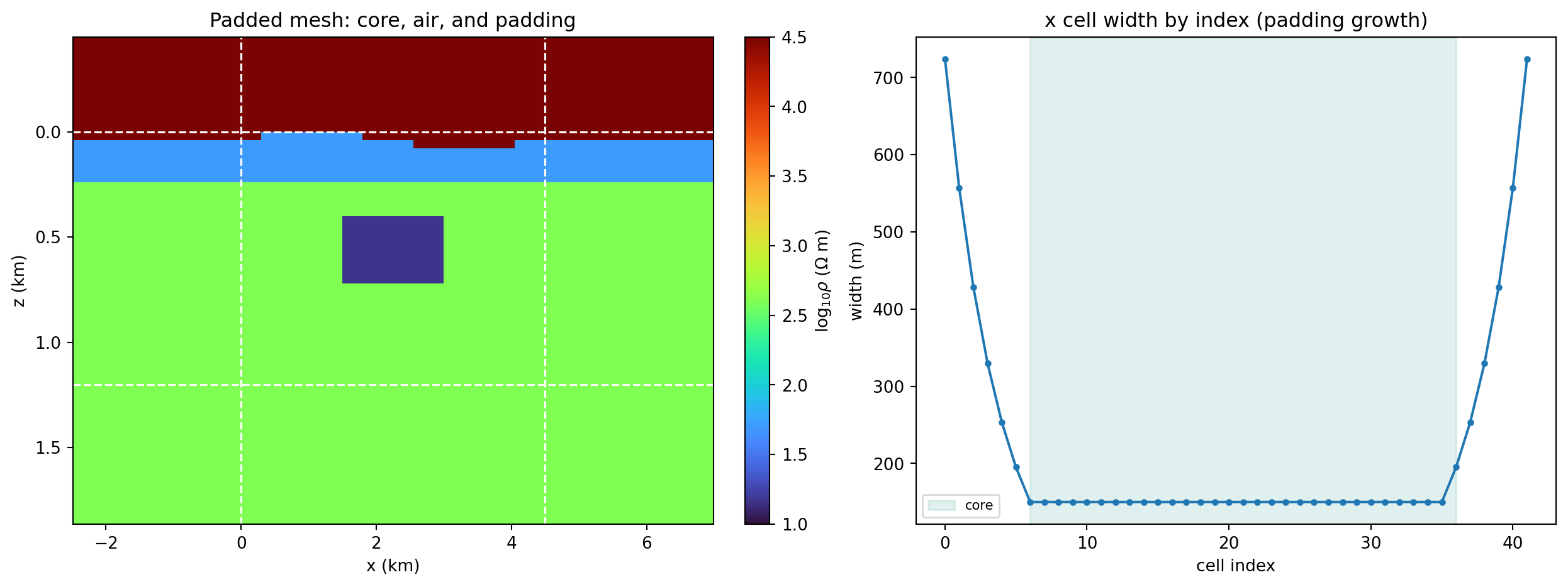
Left: the padded mesh in log-resistivity, dashed lines marking core_slices. The topographic ridge is the thin band of air cutting into the shallow conductive layer near the centre. Right: x cell width by index – flat across the shaded core, then growing geometrically into padding on both sides.

The left panel is worth reading past the colour alone. The deep-red air region sits above a visibly uneven boundary – that unevenness is the topography, rasterized onto cell centres rather than merely drawn on top of a flat mesh, and it is why the thin conductive layer just below the surface pinches and widens instead of running perfectly flat. The right panel makes the padding strategy legible in a way the mesh image alone cannot: cell width is constant across the whole shaded core, then grows smoothly outward on both flanks, each step padding_expansion times the one before it, exactly (9).

16.7.4. Skin Depth And Mesh Quality

skin_depth_m() is the standalone estimate MeshQuality scores a mesh against:

>>> round(float(skin_depth_m(40.0, 1000.0)), 1)
100.7

The mesh above is not, in fact, acceptable by its own design’s targets:

>>> model.quality.acceptable
False
>>> model.quality.warnings
('minimum skin depth has 0.919 core cells; target is 4',)

At 200 Hz over the 50 ohm m near-surface layer, the skin depth is only about 138 m – comparable to one core cell, not the four minimum_cells_per_skin_depth asks for. This is exactly the situation Maxwell Forward Modelling and Solver Contracts warns against papering over by lowering the threshold; the fix is resolution, and which axis needs it is not always obvious. Refining depth alone here does not fix it:

>>> coarse_grid = GeologyGrid.regular_2d(nx=24, nz=16, dx_m=200.0, dz_m=100.0)
>>> coarse_rho = np.full(coarse_grid.shape, 300.0)
>>> coarse_rho[:3] = 40.0
>>> small_design = MeshDesign(horizontal_padding_cells=4, bottom_padding_cells=4, air_layers=4)
>>> coarse = build_solver_mesh(
...     coarse_grid, resistivity_ohm_m=coarse_rho, frequencies_hz=[1000.0, 100.0, 10.0],
...     design=small_design,
... )
>>> coarse.quality.cells_per_minimum_skin_depth
0.5032921210448704

>>> depth_refined_grid = GeologyGrid.regular_2d(nx=24, nz=64, dx_m=200.0, dz_m=25.0)
>>> depth_refined_rho = np.full(depth_refined_grid.shape, 300.0)
>>> depth_refined_rho[:12] = 40.0
>>> depth_refined = build_solver_mesh(
...     depth_refined_grid, resistivity_ohm_m=depth_refined_rho,
...     frequencies_hz=[1000.0, 100.0, 10.0], design=small_design,
... )
>>> depth_refined.quality.cells_per_minimum_skin_depth
0.5032921210448704
>>> depth_refined.quality.warnings
('global cell-width ratio 26.6 exceeds 20', 'minimum skin depth has 0.503 core cells; target is 4')

Cutting the core cell depth from 100 m to 25 m – four times finer – changed nothing about cells_per_minimum_skin_depth, and added a second warning besides. The metric is computed from the largest core cell width across every axis, and the 200 m lateral cells never moved; refining depth alone just made the mesh more anisotropic without touching the actual bottleneck. Refining both axes together is what it takes:

>>> fine_grid = GeologyGrid.regular_2d(nx=48, nz=40, dx_m=25.0, dz_m=25.0)
>>> fine_rho = np.full(fine_grid.shape, 300.0)
>>> fine_rho[:12] = 40.0
>>> wide_design = MeshDesign(horizontal_padding_cells=6, bottom_padding_cells=6, air_layers=5)
>>> fine = build_solver_mesh(
...     fine_grid, resistivity_ohm_m=fine_rho, frequencies_hz=[1000.0, 100.0, 10.0],
...     design=wide_design,
... )
>>> fine.quality.acceptable
True
>>> fine.quality.cells_per_minimum_skin_depth
4.026336968358963

16.7.5. Near-Surface Resolution Convergence

Passing acceptable is a geometric screening gate, not proof that a solved response has actually converged – Solver-neutral Maxwell contracts already showed that by holding depth resolution fixed and varying lateral padding width, finding the half-space response barely moved at all. Holding lateral resolution fixed and refining depth resolution instead, against the closed-form layered_earth_impedance() reference for a real two-layer earth, tells the complementary story:

</>View resolution-convergence source codeClick to inspect and copy the complete code

def make_resolution_convergence() -> tuple[list[float], list[float]]:
    adapter = MT2DAdapter(verbose=False)
    frequencies = [10.0, 1.0]
    receivers = ReceiverSet([[4_000.0, 0.0]], ["S00"])
    analytic = layered_earth_impedance([100.0, 400.0], [500.0], frequencies)

    dz_values = [100.0, 50.0, 25.0, 12.5, 6.25]
    errors: list[float] = []
    cells_per_skin: list[float] = []
    for dz in dz_values:
        nz = int(round(4_000 / dz))
        grid = GeologyGrid.regular_2d(nx=40, nz=nz, dx_m=100.0, dz_m=dz)
        rho = np.full(grid.shape, 400.0)
        rho[: int(round(500 / dz))] = 100.0
        design = MeshDesign(
            horizontal_padding_cells=8, bottom_padding_cells=8, air_layers=6,
            padding_expansion=1.3, air_expansion=1.25,
        )
        model = build_solver_mesh(grid, resistivity_ohm_m=rho, frequencies_hz=frequencies, design=design)
        problem = model.to_problem(frequencies, receivers, mark_air_inactive=False)
        result = adapter.solve(problem)
        z = result.impedance_v_a[0, :, 0]
        errors.append(float(np.linalg.norm(z - analytic) / np.linalg.norm(analytic)))
        cells_per_skin.append(model.quality.cells_per_minimum_skin_depth)

    fig, ax = plt.subplots(figsize=(7, 5), constrained_layout=True)
    ax.loglog(dz_values, errors, marker="o", label="relative error vs. analytic")
    reference = errors[0] * (np.array(dz_values) / dz_values[0])
    ax.loglog(dz_values, reference, ls="--", color="black", label=r"$O(\Delta z)$ reference")
    ax.invert_xaxis()
    ax.set(title="Near-surface resolution convergence (lateral resolution fixed)",
           xlabel=r"core $\Delta z$ (m)", ylabel="relative impedance error")
    ax.legend(fontsize=9)
    ax.grid(alpha=.25, which="both")
    _save(fig, "maxwell_meshing_resolution_convergence.png")
    return errors, cells_per_skin

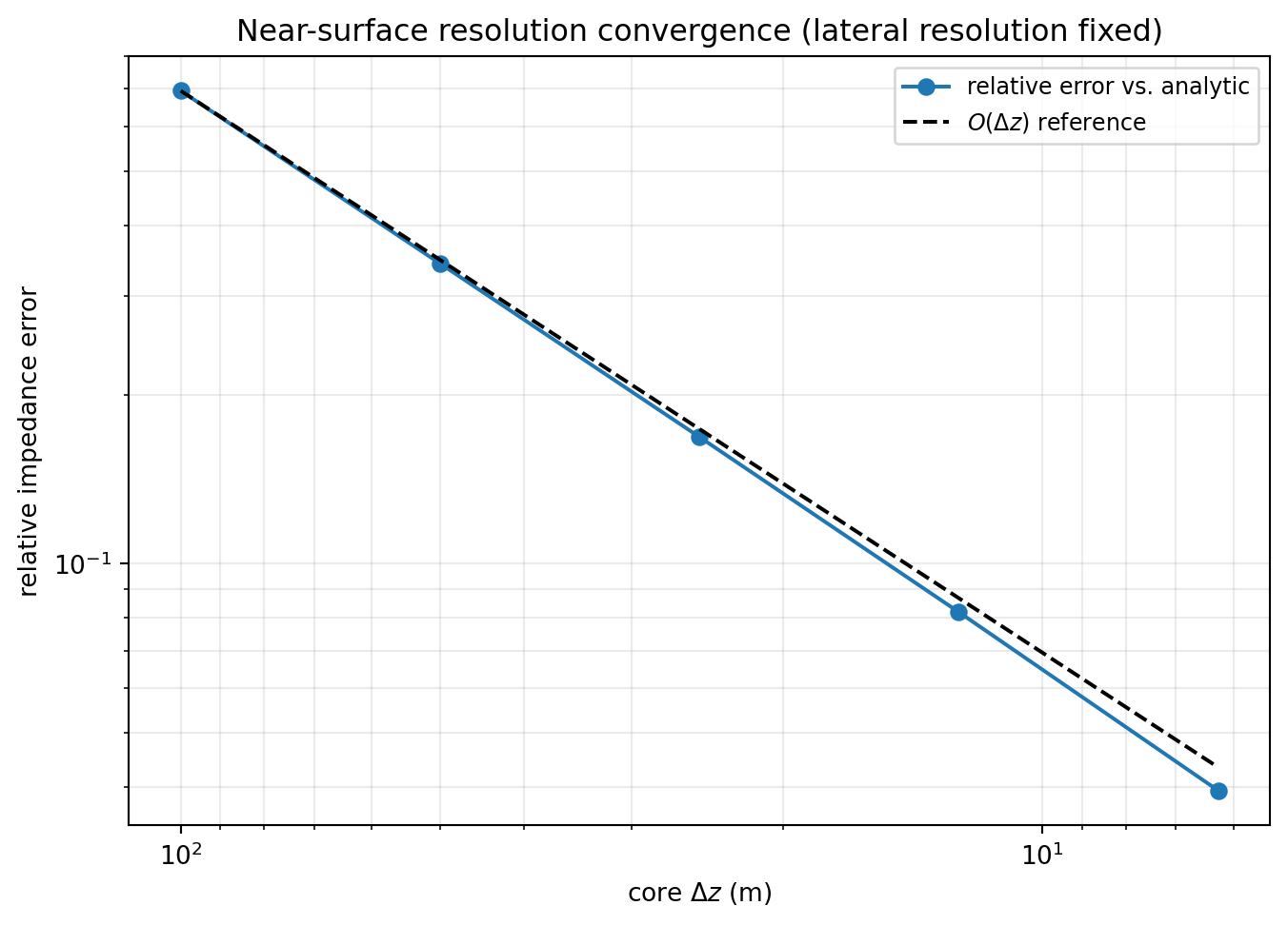
Relative impedance error at one station, against the closed-form layered-earth reference, as core dz is halved from 100 m to 6.25 m with lateral resolution held fixed throughout.

The error drops from 69% at the coarsest resolution to 4% at the finest, tracking the dashed first-order reference line closely enough on log-log axes to call this genuine, well-behaved numerical convergence rather than noise. The detail worth sitting with is what stayed constant while that happened: every one of these five meshes reported the same cells_per_minimum_skin_depth, because – exactly as in the previous section – the fixed 100 m lateral cells were the metric’s binding constraint the entire time, never the depth resolution actually being tested. An advisory geometric gate answered one question and stayed silent on the one that mattered here. Solved-response convergence, (18), is the evidence that actually closes it.

16.7.6. Receiver Placement And Terrain

assess_receivers() checks candidate receivers against the padded mesh and its terrain before to_problem() ever builds a problem from them, and each failure mode is distinct:

>>> station_x = grid.x_m[::4]
>>> receivers = ReceiverSet([[x, 0.0] for x in station_x], [f"S{i:02d}" for i in range(len(station_x))])
>>> model.assess_receivers(receivers)
()

>>> model.assess_receivers(ReceiverSet([[999_999.0, 0.0]], ["OUT"]))
('receiver x coordinates fall outside the mesh',)
>>> model.assess_receivers(ReceiverSet([[3_000.0, 500.0]], ["DEEP"]))
('receiver z coordinates fall below local terrain',)
>>> model.assess_receivers(ReceiverSet([[3_000.0, 0.0, 0.0]], ["3D"]))
('receiver and mesh dimensions differ',)

z=0 here is the reference elevation build_solver_mesh assigns to depth zero, the highest point on the ridge – everywhere else on this terrain sits at some positive depth below that shared reference, so a receiver placed at exactly z=0 is guaranteed to be on or above the local surface across the whole line, without having to interpolate the terrain by hand for every station. A station placed well below that, inside the earth rather than on it, is exactly the "DEEP" case above. to_problem() runs this same check and raises rather than silently building a problem with a buried receiver:

>>> problem = model.to_problem([20.0, 2.0], receivers, mark_air_inactive=False)
>>> problem.receivers.count
8

mark_air_inactive=False here is not a default worth overlooking: it is what makes this specific problem solvable by MT2DAdapter at all, which declares supports_inactive_cells=False and treats the whole mesh, conductive air included, as earth. Passing mark_air_inactive=True instead would build a problem only a topography-and-inactive-cell-capable adapter such as TriFEM2DAdapter or Mare2DEMAdapter could accept – Maxwell Backend Registry’s capability check exists precisely to catch that mismatch before a solve is attempted.

16.7.7. A 3-D Solver Mesh

Every mesh so far has been 2-D. build_solver_mesh builds a 3-D mesh the same way, from a 3-D GeologyGrid, with air layers and padding added on every horizontal side plus the bottom:

</>View 3-D mesh-slices source codeClick to inspect and copy the complete code

def make_3d_mesh_slices() -> tuple[tuple[int, int, int], bool]:
    grid = GeologyGrid.regular_3d(nx=22, ny=18, nz=16, dx_m=150.0, dy_m=150.0, dz_m=80.0)
    rho = np.full(grid.shape, 300.0)
    rho[:3] = 60.0
    rho[6:11, 6:12, 8:16] = 15.0
    design = MeshDesign(
        horizontal_padding_cells=5, bottom_padding_cells=5, air_layers=5,
        padding_expansion=1.3, air_expansion=1.25,
    )
    model = build_solver_mesh(grid, resistivity_ohm_m=rho, frequencies_hz=[100.0, 10.0, 1.0], design=design)
    resistivity = np.log10(1.0 / model.conductivity_s_m)
    cz, cy, cx = model.core_slices
    z_index = cz.start + 8
    y_index = cy.start + 8

    fig, axes = plt.subplots(1, 2, figsize=(13, 5), constrained_layout=True)
    x_edges, y_edges, z_edges = (model.mesh.x_edges_m / 1000, model.mesh.y_edges_m / 1000,
                                  model.mesh.z_edges_m / 1000)
    im0 = axes[0].pcolormesh(x_edges, y_edges, resistivity[z_index], cmap="turbo", shading="flat", vmin=1, vmax=3.2)
    axes[0].axvline(model.mesh.x_edges_m[cx.start] / 1000, color="white", ls="--", lw=1.1)
    axes[0].axvline(model.mesh.x_edges_m[cx.stop] / 1000, color="white", ls="--", lw=1.1)
    axes[0].axhline(model.mesh.y_edges_m[cy.start] / 1000, color="white", ls="--", lw=1.1)
    axes[0].axhline(model.mesh.y_edges_m[cy.stop] / 1000, color="white", ls="--", lw=1.1)
    axes[0].set(title=f"Horizontal slice at z={model.mesh.cell_centres_m['z'][z_index]:.0f} m",
                xlabel="x (km)", ylabel="y (km)")
    fig.colorbar(im0, ax=axes[0], label=r"$\log_{10}\rho$ ($\Omega$ m)")

    im1 = axes[1].pcolormesh(x_edges, z_edges, resistivity[:, y_index, :], cmap="turbo", shading="flat", vmin=1, vmax=3.2)
    axes[1].axvline(model.mesh.x_edges_m[cx.start] / 1000, color="white", ls="--", lw=1.1)
    axes[1].axvline(model.mesh.x_edges_m[cx.stop] / 1000, color="white", ls="--", lw=1.1)
    axes[1].axhline(model.mesh.z_edges_m[cz.start] / 1000, color="white", ls="--", lw=1.1)
    axes[1].axhline(model.mesh.z_edges_m[cz.stop] / 1000, color="white", ls="--", lw=1.1)
    axes[1].invert_yaxis()
    axes[1].set(title=f"Vertical slice at y={model.mesh.cell_centres_m['y'][y_index]:.0f} m",
                xlabel="x (km)", ylabel="z (km)")
    fig.colorbar(im1, ax=axes[1], label=r"$\log_{10}\rho$ ($\Omega$ m)")
    _save(fig, "maxwell_meshing_3d_slices.png")
    return model.mesh.shape, model.quality.acceptable

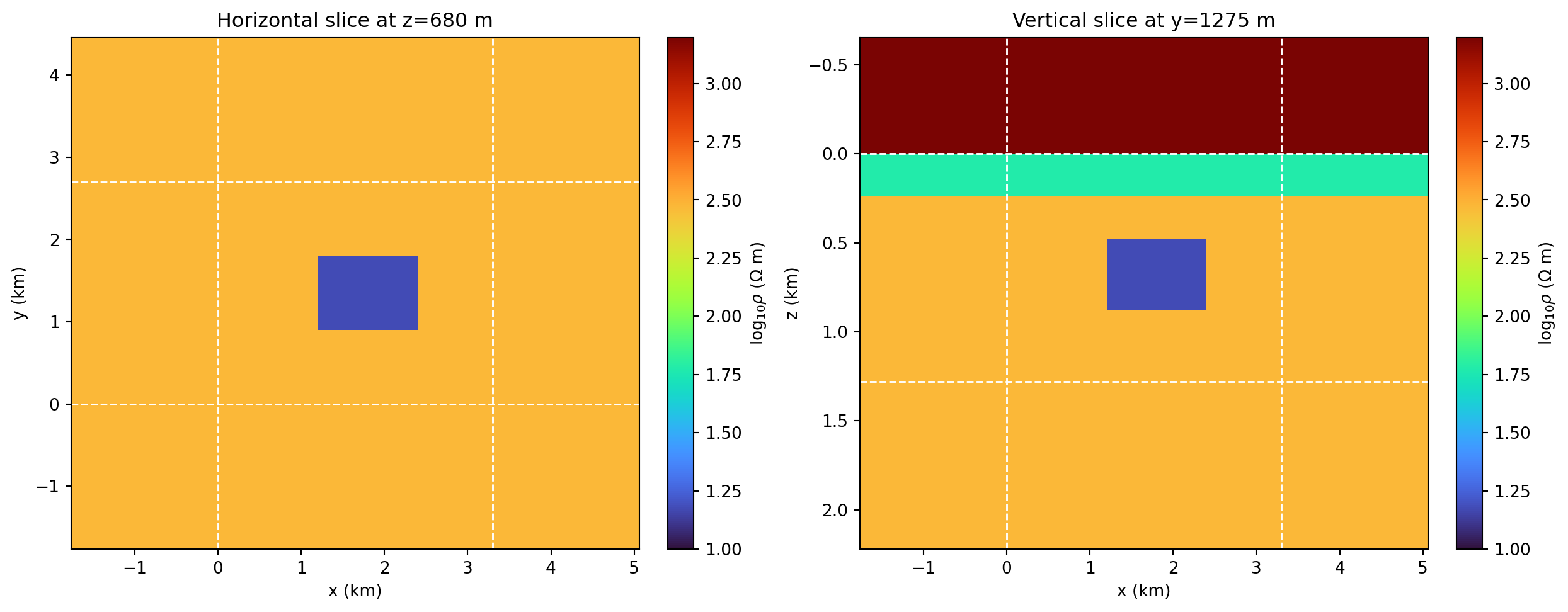
A horizontal slice through the buried target’s depth, and a vertical slice through its centre, of the same padded 3-D mesh. Dashed lines mark the core boundary on both panels.

The two slices are two views of one 26x28x32-cell mesh, not two separate models – the buried conductive block appears in both, at consistent coordinates, because both panels index the same conductivity_s_m array along different axes. The vertical slice additionally shows what the horizontal one cannot: the shallow conductive overburden as a continuous band immediately below the deep-red air region, and the true vertical separation between that overburden and the deeper, discrete target. This is exactly the mesh MT3DAdapter or ModEm3DAdapter would receive through to_problem(); a station grid instead of a single profile line is the only other change a genuine 3-D survey would add.

16.7.8. Persisting A Mesh Model

SolverMeshModel persists the same way every other contract in this package does – a compressed .npz archive, no pickle, restored through its own validated constructor:

>>> from pathlib import Path
>>> from tempfile import TemporaryDirectory
>>> directory = TemporaryDirectory()
>>> archive_path = Path(directory.name) / "model.npz"
>>> _ = model.to_npz(archive_path)
>>> restored = SolverMeshModel.from_npz(archive_path)
>>> restored.model_hash == model.model_hash
True
>>> restored.quality.acceptable == model.quality.acceptable
True

model_hash identifies the mesh, conductivity, region masks, and design together – a different MeshDesign on the identical geological grid is a different model hash, the same way a different threshold policy is a different benchmark hash in Maxwell Analytic Benchmarks even when the underlying problem is unchanged.

16.7.9. Graded Triangular Meshes

build_graded_tri_mesh takes a completely different approach: rather than padding a regular grid, it triangulates a domain boundary and receiver positions directly with Triangle, then refines that triangulation against a size function that grows triangle edge length geometrically with distance from the nearest station, capped at a maximum:

</>View triangular-grading-law source codeClick to inspect and copy the complete code

def make_tri_grading_law() -> tuple[int, float]:
    station_x = np.linspace(-500, 500, 9)
    surface_cell_m, growth_rate, max_cell_m = 20.0, 1.25, 250.0
    mesh = build_graded_tri_mesh(
        (-1_200, 1_200), (0, 900), station_x,
        surface_cell_m=surface_cell_m, growth_rate=growth_rate, max_cell_m=max_cell_m,
    )
    centroids = mesh.triangle_centroids_m
    station_points = np.column_stack([station_x, np.zeros_like(station_x)])
    distance = np.min(
        np.linalg.norm(centroids[:, None, :] - station_points[None, :, :], axis=2), axis=1,
    )
    edge_equivalent = np.sqrt(mesh.triangle_areas_m2 * 4.0 / np.sqrt(3.0))

    fig, axes = plt.subplots(1, 2, figsize=(13, 4.8), constrained_layout=True)
    triangulation = plt.matplotlib.tri.Triangulation(mesh.nodes_m[:, 0], mesh.nodes_m[:, 1], mesh.triangles)
    axes[0].triplot(triangulation, lw=0.3, color="#457b9d")
    axes[0].scatter(station_x, np.zeros_like(station_x), marker="v", color="#e76f51", zorder=5, label="stations")
    axes[0].set_ylim(500, -100)
    axes[0].set(title=f"Graded mesh, {mesh.n_triangles} triangles", xlabel="x (m)", ylabel="z (m)")
    axes[0].legend(fontsize=8)

    order = np.argsort(distance)
    axes[1].scatter(distance, edge_equivalent, s=8, alpha=.5, label="triangle equivalent edge length")
    curve_distance = np.linspace(0, distance.max(), 200)
    theoretical = np.minimum(surface_cell_m * growth_rate ** (curve_distance / surface_cell_m), max_cell_m)
    axes[1].plot(curve_distance, theoretical, color="black", ls="--", label="size function")
    axes[1].set(title="Grading law: cell size vs. distance to nearest station",
                xlabel="distance to nearest station (m)", ylabel="edge length (m)")
    axes[1].legend(fontsize=8)
    _save(fig, "maxwell_meshing_tri_grading.png")
    correlation = float(np.corrcoef(theoretical_at(distance, surface_cell_m, growth_rate, max_cell_m), edge_equivalent)[0, 1])
    return mesh.n_triangles, correlation

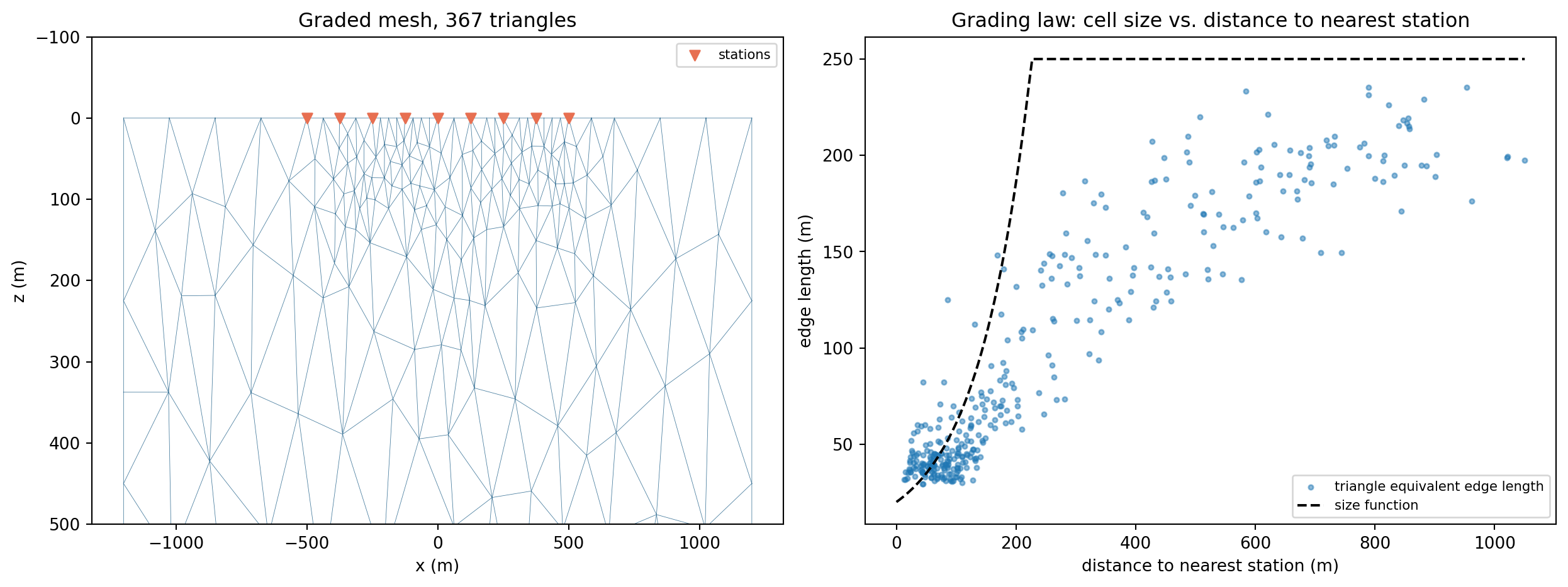
Left: the graded mesh, visibly finer directly beneath the stations. Right: every triangle’s equivalent edge length against its centroid’s distance to the nearest station, against the size function that was asked for.

The mesh panel shows the grading qualitatively – small triangles crowd the region under the stations, growing visibly coarser with depth and lateral distance. The right panel turns that impression into a real measurement: each point is one of 367 actual triangles, not a resampled curve, and it tracks the dashed size-function line with a correlation of about 0.90. Triangle’s refinement is a constraint satisfied through Ruppert’s algorithm under a simultaneous minimum-angle requirement, not an exact area assignment, so real triangles scatter around the target rather than sitting exactly on it – particularly near the cap, where the minimum-angle constraint and the area target compete most directly. A PSLG built this way still guarantees every station sits exactly on a mesh node, which TriFEM2DAdapter depends on directly.

Malformed requests are rejected before Triangle ever runs:

>>> from pycsamt.forward.maxwell import build_graded_tri_mesh
>>> build_graded_tri_mesh((0.0, 1_000.0), (0.0, 500.0), [1_500.0], surface_cell_m=20.0)
Traceback (most recent call last):
...
ValueError: station_x_m must be non-empty, finite, and within x_range_m (0.0, 1000.0).
>>> build_graded_tri_mesh((0.0, 1_000.0), (0.0, 500.0), [500.0], surface_cell_m=20.0, growth_rate=0.9)
Traceback (most recent call last):
...
ValueError: growth_rate must be finite and greater than 1.

16.7.10. Common Mistakes

Assuming cells_per_minimum_skin_depth reflects every axis

The metric is computed from the single largest core cell width across all axes. Refining one axis while another stays coarse can leave it completely unchanged, as the depth-only refinement above shows – check which axis is actually binding before refining the wrong one.

Treating quality.acceptable as proof of an accurate solve

It is an advisory geometric screen against a declared target, evaluated without ever calling a solver. The resolution-convergence study above held that metric perfectly constant while the actual solved error dropped by roughly a factor of eighteen – run Maxwell Analytic Benchmarks or a dedicated convergence study for numerical evidence, not this flag alone.

Placing receivers by guessing an elevation offset

Interpolating a topography polyline by hand to guess a receiver’s surface elevation is exactly the discretization mismatch assess_receivers exists to catch – and it will, since the mesh’s own discretized earth mask, not the smooth input surface, is what a receiver is actually checked against. Placing receivers at the shared reference depth (z=0) sidesteps the mismatch entirely whenever that convention fits the survey.

Mixing mark_air_inactive with an adapter that cannot accept it

Only backends declaring supports_inactive_cells and, for a laterally varying mask, supports_topography as well can accept a problem built with mark_air_inactive=True. Check Maxwell Backend Registry’ capability table before building the problem, not after an adapter rejects it.

Reusing a build_graded_tri_mesh region_ids convention

Every triangle gets its own region id (1..n_triangles), matching Mare2DEMAdapter’s per-triangle-region expectation. Code written against an older mesh generator that grouped many triangles under one shared region id will not carry over unchanged.

16.7.11. Next Pages

That closes the seven-page arc Maxwell Adapter Layer mapped out: contracts, meshing, the backend registry, adapters, benchmarks, and caching/batch solving all now have a real, executed page behind them. Solver-neutral Maxwell contracts and 2-D Maxwell training-data generation are the natural next stop for putting a real mesh like the ones built here to work generating training data rather than a single illustrative response.