18.7. Process Zonge AVG Lines K1 and K2#

This case study begins with the two bundled AVG file surveys and ends with reproducible classical- and AI-inversion recipes. K1 is a legacy 47-station line; K2 is a modern 28-station line. Their companion .stn files supply WGS84 / UTM Zone 49N coordinates and measured elevations. The examples use repository-relative paths and write every derived product below results/zonge_avg_tutorial; the source data are never modified.

The page concentrates on work that earlier tutorials do not repeat: legacy/modern Zonge parsing, K2 receiver-midpoint geometry, coordinate-safe AVG-to-EDI conversion, CSAMT source-effect screening, confidence-gated frequency editing, and the boundary between a scalar-line Occam2D baseline and AI inversion. Follow Prepare an Occam2D Inversion for native-file details, Run Classical Inversions: Occam2D, ModEM, and MARE2DEM for result loading, and AI Inversion From Corrected EDIs for the full AI validation audit.

18.7.1. Read the field files before converting them#

AVG normalizes both Zonge encodings into the same tidy representation. Missing values remain missing; they are not silently interpolated at read time.

>>> from pycsamt.zonge import AVG
>>> for line in ("K1", "K2"):
...     avg = AVG.from_file(f"data/avg/{line}.AVG")
...     z, freq, station = avg.to_tensor(var="z")
...     print(line, z.shape, len(freq), station.min(), station.max())
K1 (47, 17, 2, 2) 17 150.0 2450.0
K2 (28, 27, 2, 2) 27 25.0 1375.0

Both files contain only Ex-Hy, represented as \(Z_{xy}\). A zero \(Z_{yx}\) used to complete a \(2\times2\) storage array is not a second measurement. Consequently tensor skew, Groom–Bailey decomposition, strike rotation, and joint TE/TM inversion are scientifically unavailable. A function accepting the array shape does not imply that the required field components were measured.

For angular frequency \(\omega=2\pi f\), the usual SI definitions are

\[\rho_a(f) = \frac{|Z_{xy}(f)|^2}{\mu_0\omega}, \qquad \phi(f) = \operatorname{atan2}(\Im Z_{xy},\Re Z_{xy}).\]

The files retain the historical Zonge field-unit impedance convention. Do not rescale values by eye: preserve the parser’s unit metadata and compare exported EDI responses against AVG. Impedance Tensor derives the unit distinction.

18.7.2. Attach and reconcile station geometry#

K1 measurements and K1.stn share chainages. K2 is subtler: observations are at 25, 75, 125, … m, while K2.stn stores the 0, 50, 100, … m survey pegs. The observed locations are receiver midpoint positions, so equality matching would leave every K2 EDI at zero longitude and latitude. Linear interpolation is justified because every midpoint lies between measured pegs; the executable example rejects extrapolation.

>>> from docs.scripts.generate_tutorial_zonge_avg_workflow import load_line
>>> k1, k1_edis = load_line("K1")
>>> k2, k2_edis = load_line("K2")
>>> for name, avg, edis in (("K1", k1, k1_edis), ("K2", k2, k2_edis)):
...     head = edis[0].get_section("head")
...     print(name, len(edis), round(head.lat, 5), round(head.long, 5), head.elev)
K1 47 26.0524 113.48716 574.5
K2 28 25.59628 110.77275 580.5

add_topography preserves projected coordinates and elevation; convert_coords(to="ll", inplace=True) creates the geographic columns that AVGtoEDI writes into EDI HEAD and DEFINEMEAS. EPSG:32649 is this dataset’s provenance, not a universal default. Use the field crew’s verified CRS for another survey.

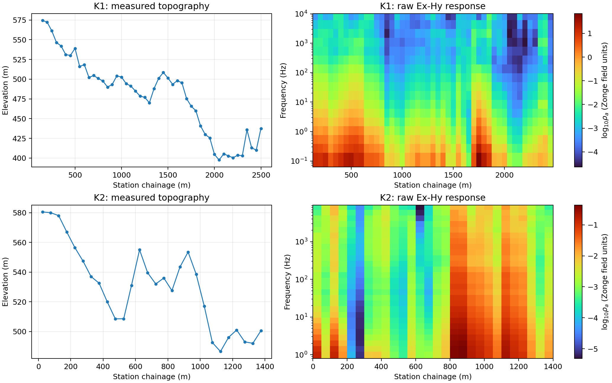
K1 and K2 measured topography and raw Ex-Hy apparent-resistivity pseudosections. — K1 crosses about 177 m of relief over 2.3 km; K2 crosses about 94 m over 1.35 km after midpoint interpolation. Broad structure persists through adjacent frequencies, whereas isolated cells and edge bands need QC. Frequency increases upward, placing the shallow-sensitive high-frequency response at the top and the deeper-sensitive low-frequency response at the bottom; frequency is a sensitivity scale, not a literal depth coordinate. Colours are raw Zonge field-unit responses, not a resistivity model.#

18.7.3. Preview coordinate-bearing EDI serialization#

This early write/read round trip verifies the transformer and coordinates; it does not yet nominate the inversion input. Write each line separately and fail if any station cannot be serialized.

>>> from pathlib import Path
>>> root = Path("results/zonge_avg_tutorial")
>>> for name, collection in (("K1", k1_edis), ("K2", k2_edis)):
...     report = collection.export(root / "edi_raw" / name)
...     if report["failed"]:
...         raise RuntimeError(report["failed"])
...     print(name, len(report["successful"]), "EDI files")
K1 47 EDI files
K2 28 EDI files

Read the files back rather than trusting only in-memory objects. lines is the immutable raw-EDI control mapping used below:

>>> from pycsamt.emtools import ensure_sites
>>> lines = {
...     name: ensure_sites(root / "edi_raw" / name, recursive=False).ordered()
...     for name in ("K1", "K2")
... }
>>> [(name, len(sites)) for name, sites in lines.items()]
[('K1', 47), ('K2', 28)]

Compare first and last EDI coordinates with topo.frame and confirm every latitude, longitude, elevation, frequency, and complex \(Z_{xy}\) value is finite wherever AVG was finite. Transformers explains the lower-level naming, unit, and section-writing contracts.

18.7.4. Choose processing from evidence#

Begin with native AVG QC because it retains %Rho, phase scatter, and electric/magnetic errors that a reduced EDI may not preserve:

pycsamt avg validate data/avg/K1.AVG --top 15
pycsamt avg validate data/avg/K2.AVG --top 15
pycsamt avg stations data/avg/K2.AVG --stn-file data/avg/K2.stn

The figure below was computed directly from all 1,555 AVG rows. It is more informative than a generic full-tensor confidence score because these scalar files have no measured \(Z_{yx}\). Such a score would incorrectly treat the absent component as an off-diagonal mismatch.

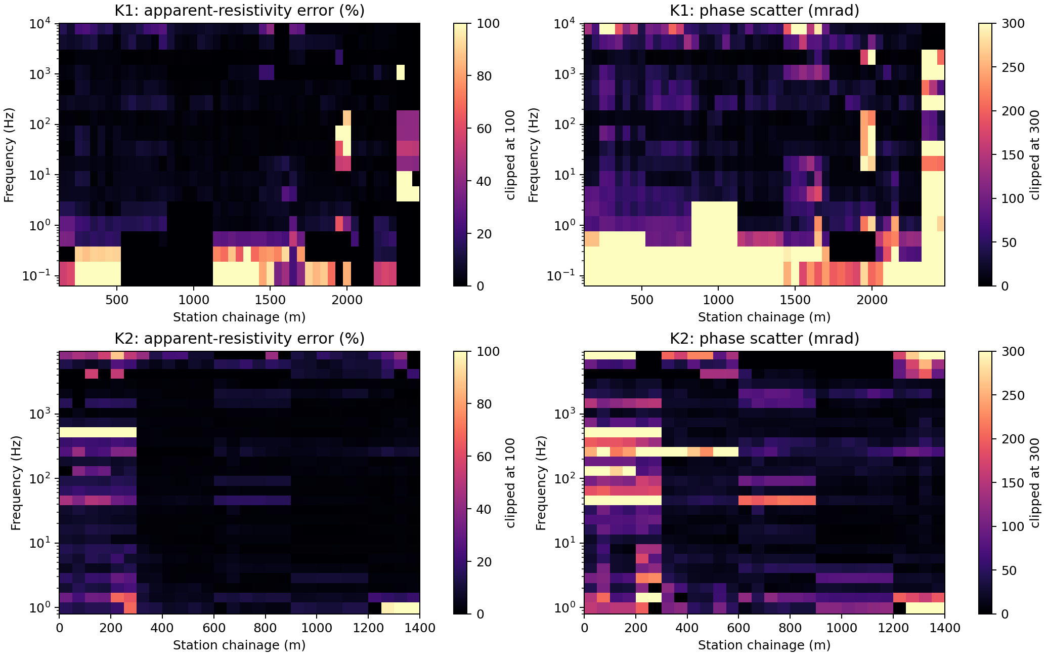
Native apparent-resistivity percentage error and phase scatter for K1 and K2. — K1 has median `%Rho=3.0` and median phase scatter `34.4 mrad`; its 90th percentiles rise to `29.22%` and `545.2 mrad`. K2 has medians `2.5%` and `22.1 mrad` and 90th percentiles `17.15%` and `152.9 mrad`. The long-period/high-scatter patches and isolated vertical bands should be reviewed before any global frequency rejection. Values are clipped only for display; the calculations retain their full magnitude.#

This supports a scalar-safe mask based on the recorded uncertainties. Keep the original rows and attach a reason rather than deleting them immediately:

>>> import numpy as np
>>> reviewed_avg = {}
>>> for name in ("K1", "K2"):
...     avg = AVG.from_file(f"data/avg/{name}.AVG")
...     frame = avg.df.copy()
...     frame["review_reason"] = ""
...     bad_rho = frame["pc_rho"].gt(50.0)
...     bad_phase = frame["s_phz"].gt(300.0)
...     frame.loc[bad_rho, "review_reason"] += "rho_error>50%;"
...     frame.loc[bad_phase, "review_reason"] += "phase_scatter>300mrad;"
...     reviewed_avg[name] = frame
...     print(name, "review rows:", int((bad_rho | bad_phase).sum()))
K1 review rows: 139
K2 review rows: 38

The thresholds are explicit first-pass gates, not automatic truth. Review curves at the flagged station-frequency pairs and revise them with field notes. edit_frequencies_by_confidence() is appropriate for genuine two-component MT data, but its off-diagonal term is not an admissible decision rule for these Ex-Hy-only lines.

18.7.4.1. Run and inspect a static-shift trial#

ASTATIC can execute Zonge-style spatial filtering before EDI export. The following trial was run on fresh copies of both AVG objects, using the highest shared frequency and a five-station trimmed moving average. It never mutates the bundled files.

>>> from pycsamt.zonge.processing import ASTATIC
>>> trials = {}
>>> for name in ("K1", "K2"):
...     raw = AVG.from_file(f"data/avg/{name}.AVG")
...     ref = float(raw.df.freq.max())
...     proc = ASTATIC().read(raw)
...     shifts = proc.correct_static_shift(
...         reference_freq=ref, filter_method="tma",
...         window_size=5, update_components=True,
...     )
...     trials[name] = (proc.avg, shifts)
...     print(
...         name, ref,
...         round(float(shifts.shift_factor.min()), 3),
...         round(float(shifts.shift_factor.max()), 3),
...         round(float(shifts.shift_factor.median()), 3),
...     )
K1 8192.0 0.102 14.507 1.403
K2 8192.0 0.13 45.665 1.157

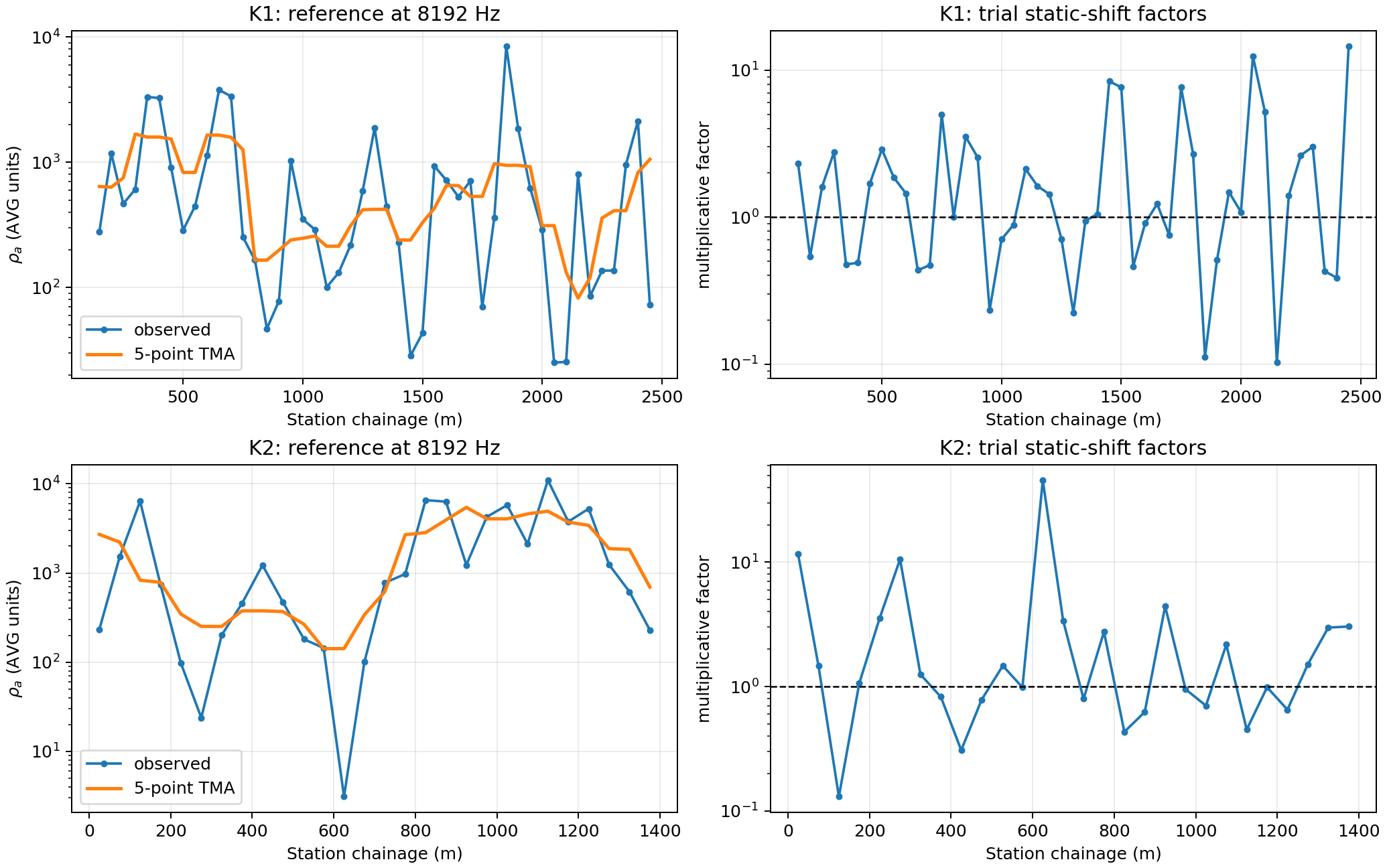
Observed and five-point TMA reference-frequency profiles and inferred static-shift factors for K1 and K2. — The trial does not justify accepting the correction. K1 factors span about 0.10–14.51 and K2 spans 0.13–45.67; the latter is driven partly by the 625 m station’s very small reference-frequency response. Median absolute changes are 0.327 and 0.271 log10 decades respectively. Factors this extreme say that the chosen high-frequency reference is unstable or strongly structured, not automatically that geology-free static shift has been isolated. Compare reference frequencies and window sizes, inspect native errors, and retain the raw line as the Occam2D control run.#

Capacitive-coupling correction is not run because the method requires measured electrode contact resistance, setup length, and wire capacitance; none is present in the bundled files. Supplying convenient constants would produce an image, but not a reproducible correction.

The Zonge decision is therefore explicit: neither the extreme 8192 Hz static trial nor an undocumented capacitive correction is accepted. The selected AVG product for both lines is the coordinate-attached, otherwise unmodified AVG object already transformed and round-trip checked above. This is not a failure to process; it is a processing decision supported by the captured diagnostics. lines now becomes the starting point for applicable EDI conditioning.

18.7.4.2. Screen controlled-source effects without inventing geometry#

Two additional pycsamt.emtools diagnostics are relevant, but cannot be executed honestly from these four files alone. With skin depth \(\delta_B\simeq356\sqrt{\rho_a/f}\) m and source distance \(r\), the dimensionless \(|kr|\propto r/\delta_B\) separates near, transition, and far fields. classify_field_zones() and detect_source_overprint() require the surveyed transmitter-to-receiver offsets. Supply them from the field record; never infer them from receiver chainage:

>>> from pycsamt.emtools import classify_field_zones, detect_source_overprint
>>> # Define from the external transmitter survey before running this block.
>>> source_offsets_m = {s.name: measured_offset[s.name] for s in lines["K1"]}
>>> zones = classify_field_zones(lines["K1"], source_offset=source_offsets_m)
>>> overprint = detect_source_overprint(
...     lines["K1"], source_offset=source_offsets_m
... )

measured_offset is deliberately undefined: bundled AVG/STN files lack defensible transmitter coordinates. A source-effect figure or correction without that observation would be fabricated. Do not use tensor-only anisotropy, skew, strike, or off-diagonal consistency on these inputs either.

18.7.4.3. Process the converted EDIs and export the inversion input#

The accepted, executable EDI sequence is deliberately short and compatible with the one measured Ex-Hy component:

a frequency-domain Hampel filter in magnitude/phase space detects isolated response spikes without smoothing every datum;
the Torres–Verdín–Bostick Hanning spatial correction estimates static shift from \(Z_{xy}\) only, over a 500 m window;
corrected EDIs and a coordinate manifest are written, reloaded, and counted before either inversion sees them.

>>> from pycsamt.emtools import correct_static_shift, hampel_filter_freq
>>> from pycsamt.site.export import write_sites
>>> corrected_lines = {}
>>> for name, raw_sites in lines.items():
...     despiked = hampel_filter_freq(
...         raw_sites, win=2, nsig=3.0, on="z",
...         domain="magphase", inplace=False,
...     )
...     corrected = correct_static_shift(
...         despiked, window_m=500.0, spacing_m=50.0,
...         comp="xy", inplace=False,
...     )
...     out = root / "edi_corrected" / name
...     paths = write_sites(
...         corrected, out, exist_ok=True,
...         manifest_csv=out / "manifest.csv",
...     )
...     corrected_lines[name] = ensure_sites(out).ordered()
...     print(name, len(paths), len(corrected_lines[name]))
K1 47 47
K2 28 28

The code was executed through the reusable generator. Hampel despiking changed 25 K1 station-frequency cells and 7 K2 cells; its median absolute change is zero because most observations are deliberately preserved. The following panels show every change introduced by each operation rather than only the more attractive corrected response.

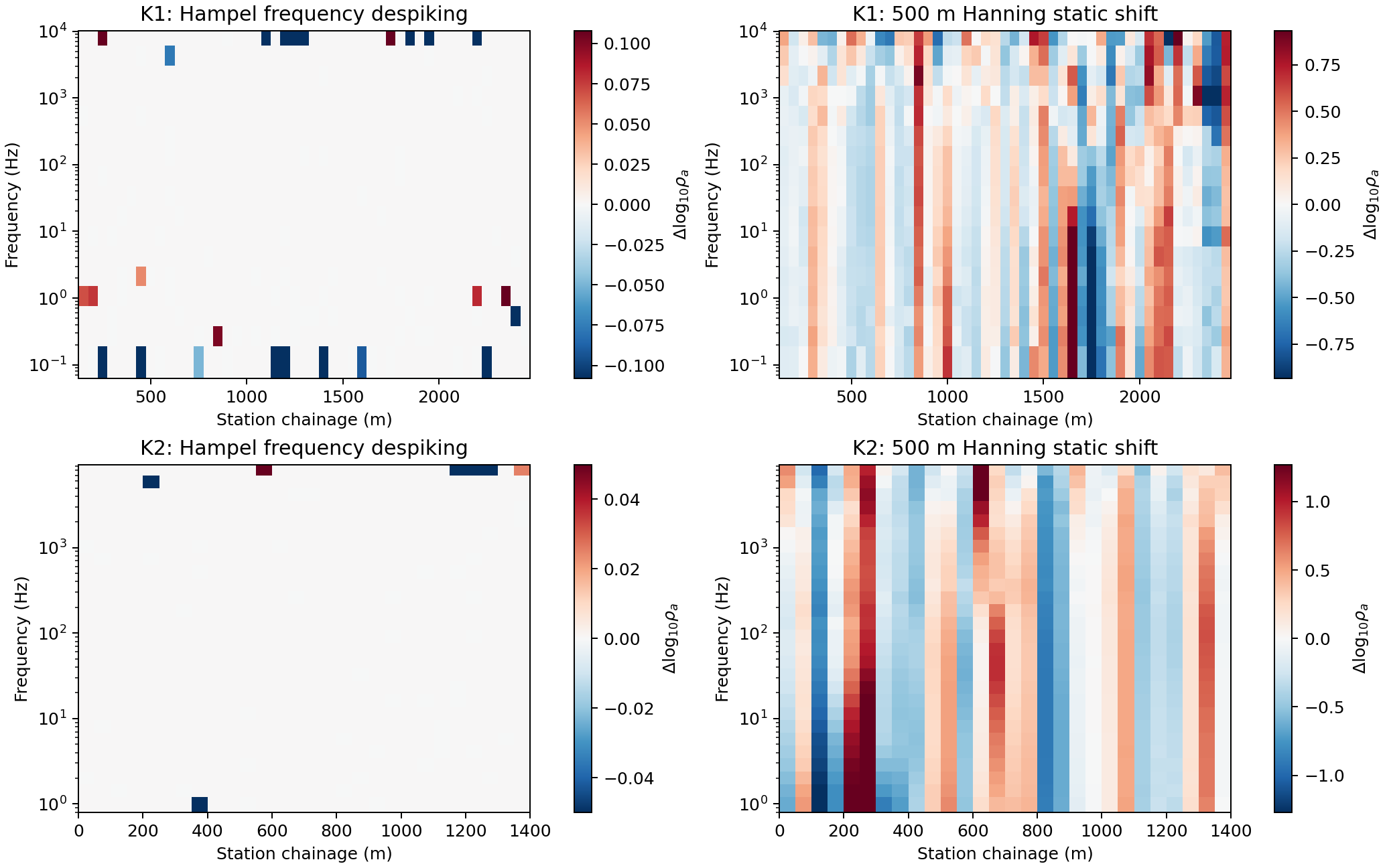
Changes in log apparent resistivity introduced by EDI Hampel despiking and Hanning static-shift correction for K1 and K2. — Frequency despiking is sparse, concentrated at isolated edge-band cells. The spatial correction is much broader: median absolute changes are 0.213 log10 decades for K1 and 0.358 for K2, with some stations exceeding one decade. That scale requires a sensitivity run with wider windows and an uncorrected control inversion. The files are technically valid corrected EDIs, but processing provenance—not the filename—determines whether they are acceptable for interpretation.#

View the complete executed EDI processing, export, reload, and plotting codeClick to inspect and copy the complete code

def make_edi_processing(lines):
    """Run the scalar-safe EDI processing chain and export corrected EDIs."""
    from pycsamt.emtools import hampel_filter_freq
    from pycsamt.emtools._core import ensure_sites
    from pycsamt.site.export import write_sites

    fig, axes = plt.subplots(2, 2, figsize=(11.5, 7.2), constrained_layout=True)
    summaries = []
    corrected_lines = {}
    for row, (name, _avg, raw) in enumerate(lines):
        despiked = hampel_filter_freq(
            raw, win=2, nsig=3.0, on="z", domain="magphase", inplace=False
        )
        corrected = process_edi_collection(raw)
        corrected_lines[name] = corrected
        chain, freq, rho0 = _edi_rho_matrix(raw)
        _, _, rho1 = _edi_rho_matrix(despiked)
        _, _, rho2 = _edi_rho_matrix(corrected)
        tiny = np.finfo(float).tiny
        d_hampel = np.log10(np.maximum(rho1, tiny)) - np.log10(np.maximum(rho0, tiny))
        d_static = np.log10(np.maximum(rho2, tiny)) - np.log10(np.maximum(rho1, tiny))
        for col, (delta, title) in enumerate(
            ((d_hampel, "Hampel frequency despiking"),
             (d_static, "500 m Hanning static shift"))
        ):
            lim = max(0.05, float(np.nanpercentile(np.abs(delta), 98)))
            pc = axes[row, col].pcolormesh(
                chain, freq, delta.T, shading="auto", cmap="RdBu_r",
                vmin=-lim, vmax=lim,
            )
            axes[row, col].set_yscale("log")
            # Keep high frequencies at the top, consistent with make_overview:
            # they are generally more sensitive to shallow structure.
            axes[row, col].set(title=f"{name}: {title}",
                               xlabel="Station chainage (m)", ylabel="Frequency (Hz)")
            fig.colorbar(pc, ax=axes[row, col], label=r"$\Delta\log_{10}\rho_a$")

        outdir = ROOT / "results" / "zonge_avg_tutorial" / "edi_corrected" / name
        paths = write_sites(
            corrected, outdir, exist_ok=True,
            manifest_csv=outdir / "manifest.csv",
        )
        reloaded = ensure_sites(outdir, recursive=False).ordered()
        summaries.append(
            (name, int(np.sum(np.abs(d_hampel) > 1e-12)),
             float(np.nanmedian(np.abs(d_hampel))),
             float(np.nanmedian(np.abs(d_static))), len(paths), len(reloaded))
        )
    target = OUT / "k1_k2_edi_processing_changes.png"
    fig.savefig(target, dpi=180); plt.close(fig)
    return target, corrected_lines, summaries

From this point onward, corrected_lines is the sole input mapping used by the inversion examples. Keep lines unchanged for raw-versus-corrected control runs.

18.7.4.4. Compare station responses before tensor diagnostics#

A line-wide change map can hide a poor curve at one receiver. The public one-dimensional plotting API therefore checks the first, middle, and last station of each line. raw=True deliberately selects the black raw-data style and draws the imported uncertainty bars; raw=False uses the normal pyCSAMT component style for the corrected values.

>>> from pycsamt.emtools import plot_raw_sites_1d
>>> for name in ("K1", "K2"):
...     station_names = [site.station for site in lines[name]]
...     selected = [station_names[0], station_names[len(station_names)//2],
...                 station_names[-1]]
...     raw_figure = plot_raw_sites_1d(
...         lines[name], stations=selected, components=("xy",),
...         raw=True, show_error_bars=True, ncols_groups=3,
...     )
...     corrected_figure = plot_raw_sites_1d(
...         corrected_lines[name], stations=selected, components=("xy",),
...         raw=False, show_error_bars=True, ncols_groups=3,
...     )
...     print(name, selected)
K1 ['S150', 'S1300', 'S2450']
K2 ['S025', 'S725', 'S1375']

Raw apparent resistivity and phase with error bars at three K1 stations.

Corrected apparent resistivity and phase at the same three K1 stations.

Raw apparent resistivity and phase with error bars at three K2 stations.

Corrected apparent resistivity and phase at the same three K2 stations.

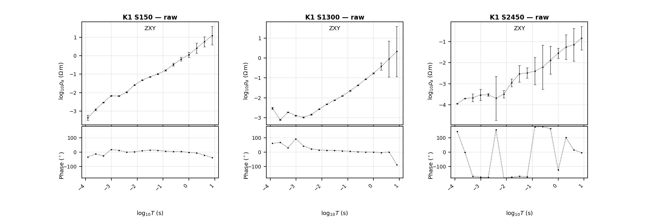
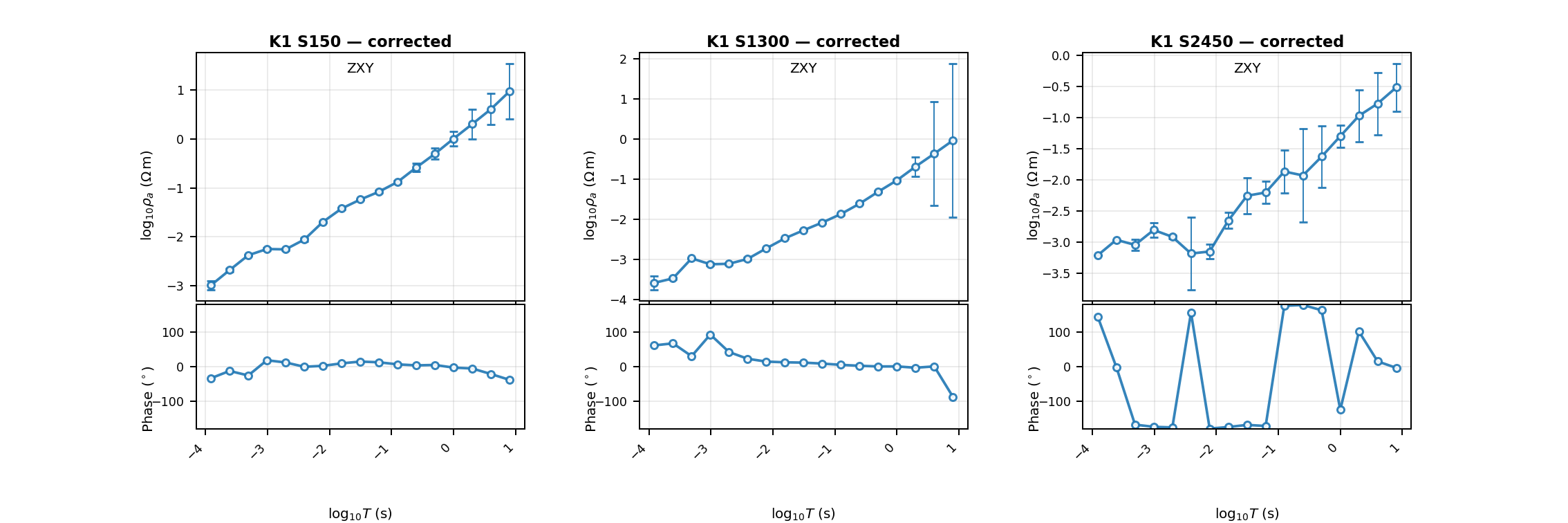
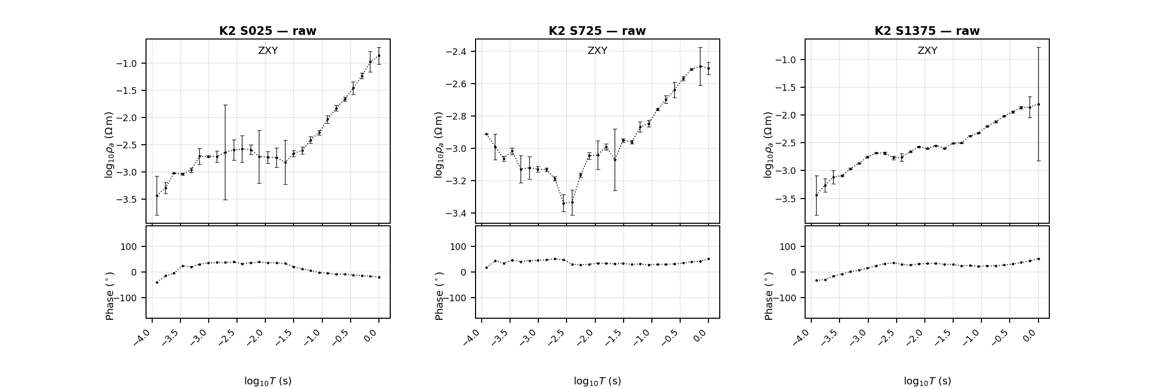
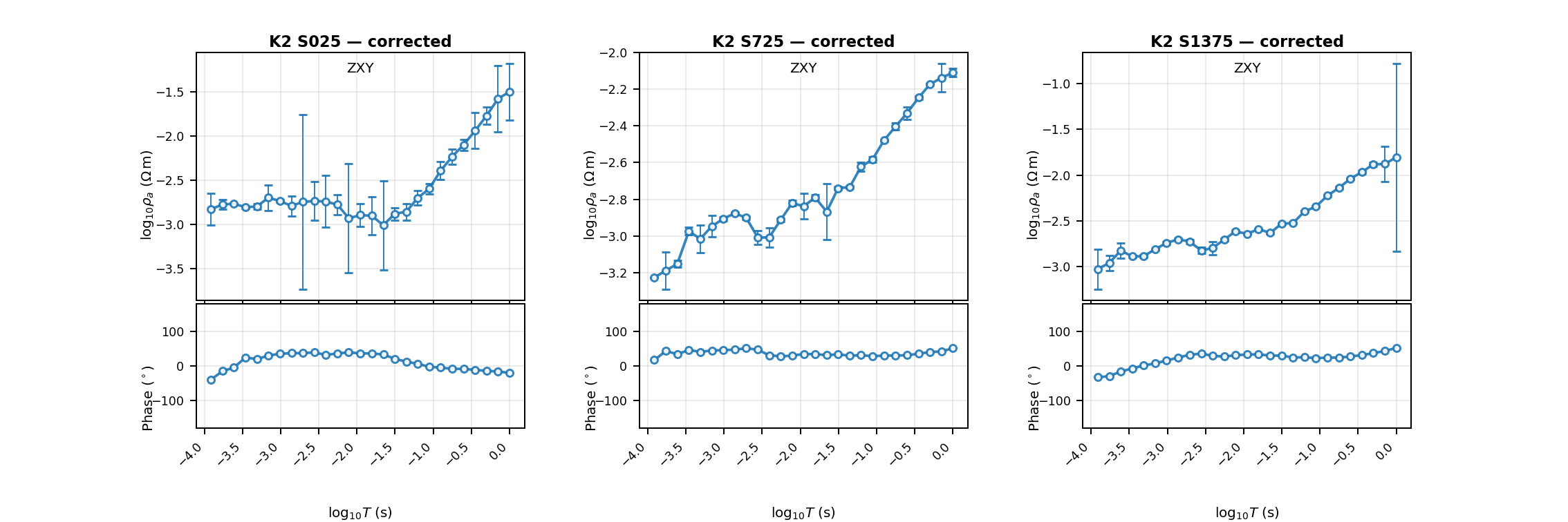
The end stations expose the strongest phase wrapping and the largest reported resistivity errors. The corrected curves retain their broad period trends, while isolated spikes and station-wise level offsets change. This is the expected signature of the chosen two-stage processing; a correction that instead erased a broad phase transition would be grounds to reject it.

18.7.4.5. Decide whether phase-tensor rotation is supported#

The phase tensor is not computed element by element. It requires the complete complex impedance tensor,

\[\boldsymbol{\Phi}(\omega) =[\operatorname{Re}\mathbf Z(\omega)]^{-1} \operatorname{Im}\mathbf Z(\omega).\]

Thus the real part must be an invertible 2x2 matrix. K1 and K2 measured only Ex–Hy, stored as \(Z_{xy}\). The other three EDI cells are storage zeros, not observations, so \(\operatorname{Re}\mathbf Z\) is singular. A phase ellipse, tensor skew, or geoelectric strike calculated from it would be fabricated.

>>> # Captured while auditing the converted EDI collections.
>>> for name, bearing, measured in tensor_audit:
...     print(f"{name}: measured components {measured}/4; profile bearing {bearing:.1f} deg")
K1: measured components 1/4; profile bearing 125.8 deg
K2: measured components 1/4; profile bearing 120.9 deg

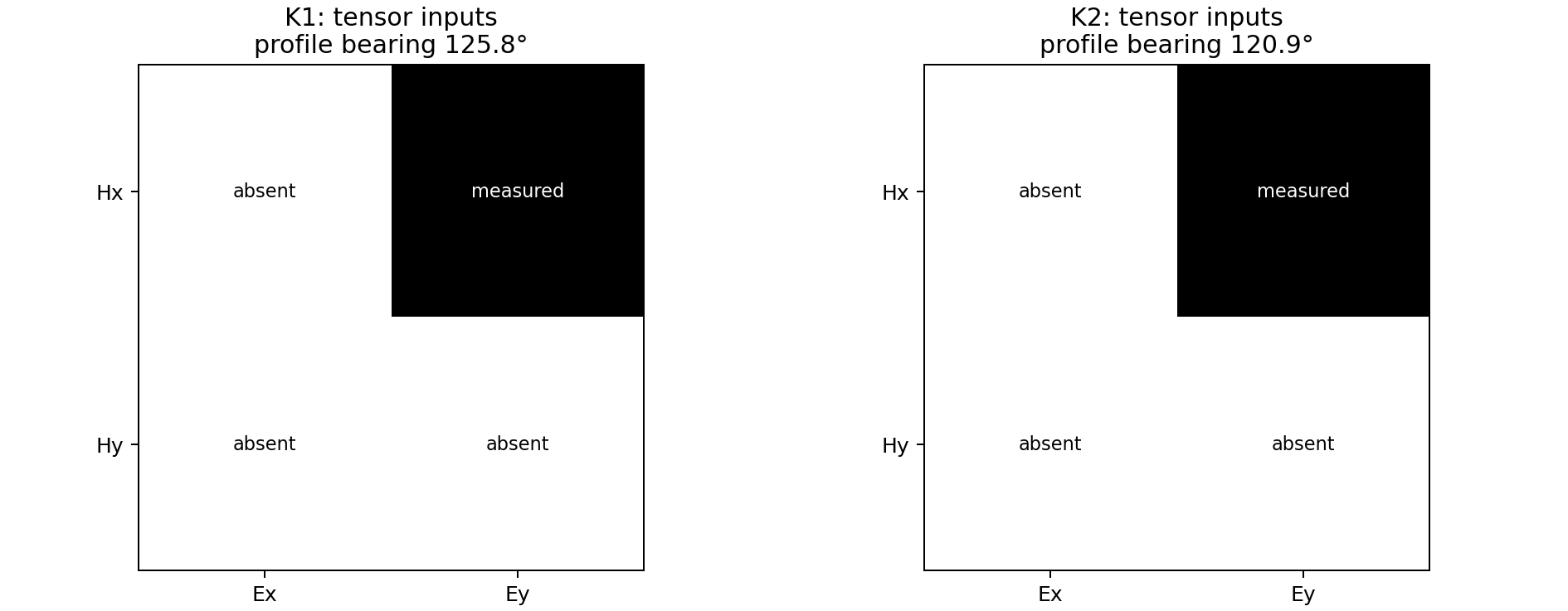
Both lines contain only the Ex–Hy transfer function. Their similar southeast profile bearings describe acquisition direction, not subsurface lineament direction; no impedance rotation is justified for these data.#

When a future survey supplies all four measured components, the corresponding emtools workflow is:

>>> from pycsamt.emtools import (
...     estimate_strike_consensus, plot_phase_tensor_strip_grid,
...     plot_strike_analysis, rotate_to_strike,
... )
>>> full_tensor_lines = {"K1": k1_full, "K2": k2_full}  # measured XX, XY, YX, YY
>>> ellipse_stations = {
...     name: [site.station for site in sites][::max(1, len(sites)//6)]
...     for name, sites in full_tensor_lines.items()
... }
>>> all_full_tensor_sites = list(k1_full) + list(k2_full)
>>> fig = plot_phase_tensor_strip_grid(
...     all_full_tensor_sites, profiles=ellipse_stations,
... )
>>> for name, sites in full_tensor_lines.items():
...     strike = estimate_strike_consensus(sites, band=(0.01, 10.0))
...     strike_fig = plot_strike_analysis(sites, method="consensus")
...     rotated = rotate_to_strike(
...         sites, method="consensus", band=(0.01, 10.0), inplace=False,
...     )
...     write_sites(rotated, root / "edi_rotated" / name, exist_ok=True)

Inspect ellipse coherence, skew, strike ambiguity, and frequency stability before accepting that rotation. For the bundled K1/K2 realization the decision is instead do not rotate: proceed with the measured \(Z_{xy}\) as a single-mode baseline and carry the missing-tensor limitation into the interpretation.

18.7.5. Prepare the classical Occam2D baseline#

Occam2D minimizes a regularized objective such as

\[\Phi(m;\lambda)=\|W_d[d-F(m)]\|_2^2 +\lambda^2\|W_m(m-m_{\rm ref})\|_2^2,\]

where \(d\) is reviewed data, \(F(m)\) the forward response, \(W_d\) inverse uncertainty, and \(W_m\) model roughness. An error floor prevents noise from receiving excessive weight. Since K1/K2 contain only \(Z_{xy}\), build TE-only; TE+TM would imply data that do not exist.

>>> from pycsamt.models.occam2d import OccamConfig, InputBuilder
>>> for name, sites in corrected_lines.items():
...     workdir = root / "occam2d" / name
...     cfg = OccamConfig(
...         modes=["TE"], error_floor_rho=0.07,
...         error_floor_phase=1.0, n_layers=32,
...         cell_size_horizontal=50.0, cell_size_vertical_top=20.0,
...         target_misfit=1.0, max_iterations=80, initial_rho=100.0,
...     )
...     cfg.to_template(workdir / "occam2d.yml")
...     builder = InputBuilder(sites, workdir=workdir, config=cfg, verbose=1)
...     builder.build(title=f"{name} Zonge AVG TE Occam2D baseline")
...     print(name, builder.summary())

The floors are transparent starting values and must be compared with AVG uncertainties. Review all four native files as shown in Prepare an Occam2D Inversion before launching anything.

18.7.6. Compile and run on the user’s machine#

pyCSAMT integrates source; it does not ship a compiled binary. Prerequisites and platform notes are at Occam2D in Compiling the External Solvers:

pycsamt build occam2d --auto-install -y
pycsamt build occam2d --status

After validating each directory, launch explicitly:

>>> from pycsamt.models.occam2d import OccamRunner
>>> binary = "/absolute/path/to/Occam2D"  # Occam2D.exe on Windows
>>> for name in ("K1", "K2"):
...     runner = OccamRunner(
...         workdir=root / "occam2d" / name, binary_path=binary,
...         startup_file="Startup", verbose=1,
...     )
...     code = runner.run(max_iter=80, target_misfit=1.0, auto_compile=False)
...     if code != 0:
...         raise RuntimeError(f"{name}: Occam2D exit code {code}")

No K1/K2 inversion result is claimed here because no external binary was invoked. Once run, inspect RMS, roughness, residuals, and mesh sensitivity with Run Classical Inversions: Occam2D, ModEM, and MARE2DEM; a colourful section is not validation.

18.7.7. Train an AI counterpart, not a replacement baseline#

Build a geological prior and Maxwell dataset whose extent, sampling, frequency band, depth, and resistivity support are recorded per line. K1 and K2 must be trained independently because they have different station counts and spatial support. The executed tutorial realization uses each line’s corrected EDIs, 32 independent 2-D Maxwell profiles, five frequencies, eight depth cells, and at most 50 epochs with validation early stopping. This is stronger than a one-line smoke test and checks both complete data contracts, but remains an audit-sized training budget.

>>> from docs.scripts.generate_tutorial_zonge_avg_workflow import make_ai_two_line
>>> path, ai_results = make_ai_two_line(corrected_lines)
>>> for name, result in ai_results.items():
...     recovery = result.data["mt2d_recovery"]
...     epochs_run = len(result.data["inverter"]._history["train_loss"])
...     print(name, result.status, round(result.data["rms_global"], 3),
...           round(recovery["rmse"], 3), round(recovery["r2"], 3),
...           epochs_run)
K1 success 4.891 0.801 -0.004 9
K2 success 4.726 0.806 -0.017 12

The learning objective combines supervised error and spatial regularizers,

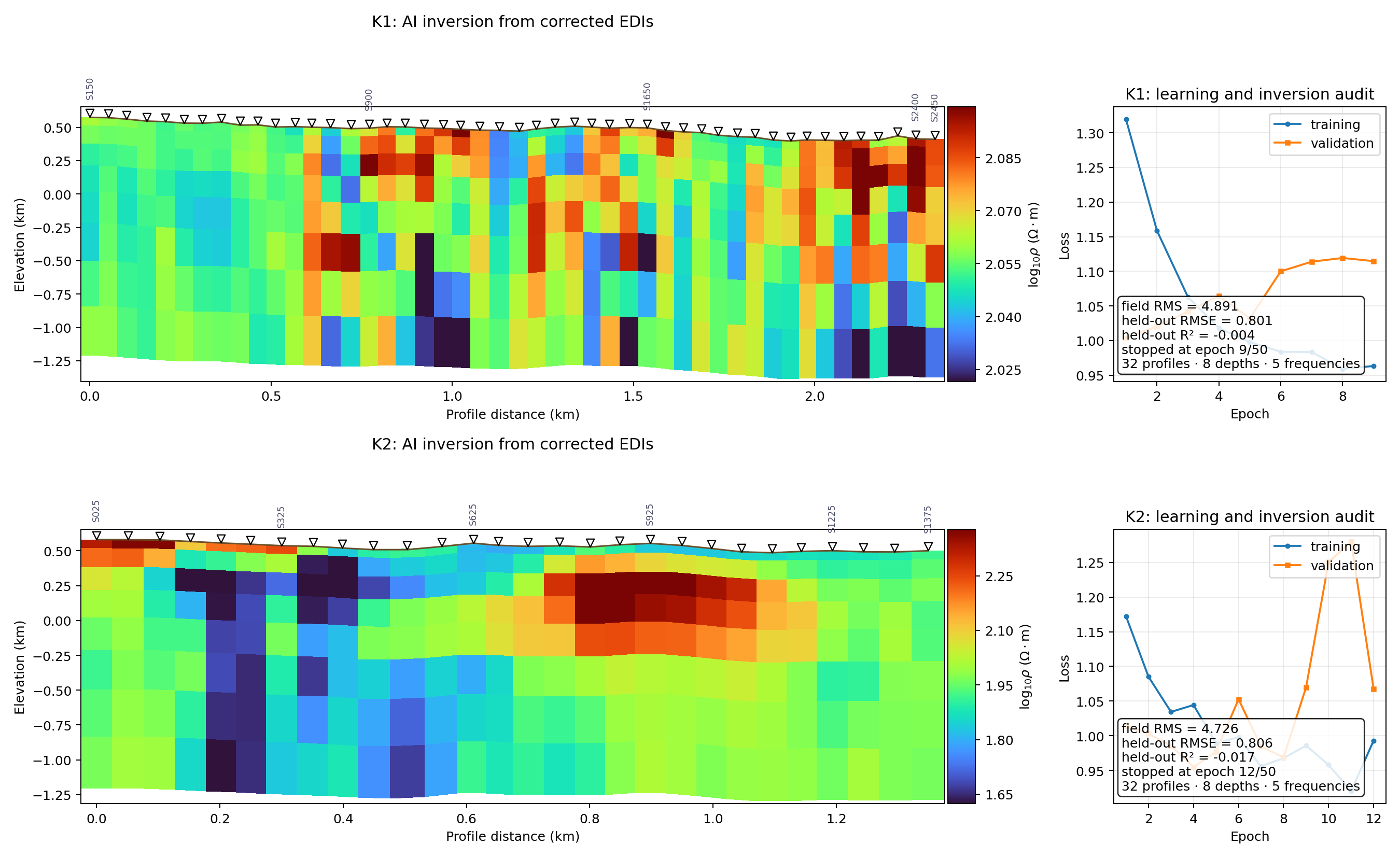
\[\mathcal L=\mathcal L_{\rm data} +\lambda_x\|\nabla_xm\|_1+\lambda_z\|\nabla_zm\|_1 +\lambda_{\rm TV}\operatorname{TV}(m).\]

Executed K1 and K2 topography-draped AI inversions with learning and recovery audits. — Each row uses columns one and two for the inversion section and column three for its learning and inversion audit. The shared topography renderer places station markers and selected station labels above the measured surface. Fifty is an upper bound rather than a target: `patience=8` stops a line when validation loss has not improved for eight consecutive epochs and restores the best validation checkpoint. With 32 profiles per line, K1 stopped after 9 epochs and K2 after 12. This prevents the falling training loss and rising validation loss seen when all 50 epochs were forced. Increasing the profile count alone did not improve held-out recovery: both \(R^2\) values remain approximately zero. The remaining problem is therefore not merely sample count; the synthetic resistivity prior, noise model, frequency support, and Maxwell-to-field domain match need improvement. Early stopping limits damage but cannot repair an unrepresentative training distribution. Apparent coloured bodies still require acceptable field residuals and held-out recovery before they can be interpreted as geology.#

View the executed two-line Maxwell training, topography, and audit codeClick to inspect and copy the complete code

def make_ai_two_line(corrected_lines):
    """Train independent K1/K2 models and render topographic audit rows."""
    from pycsamt.agents import Inv2DAgent
    from pycsamt.topo import plot_topo_section

    np.random.seed(20260803)
    try:
        import torch
        torch.manual_seed(20260803)
    except ImportError:
        pass
    freqs = np.array([32.0, 128.0, 512.0, 2048.0, 8192.0])
    results = {}
    for index, name in enumerate(("K1", "K2")):
        np.random.seed(20260803 + index)
        try:
            torch.manual_seed(20260803 + index)
        except (ImportError, NameError):
            pass
        sites = corrected_lines[name]
        agent = Inv2DAgent(
            physics="mt2d", n_depth=8,
            n_stations_per_profile=len(sites), n_train_profiles=32,
            epochs=50, patience=8, depth_max=1600.0,
            station_spacing_m=50.0,
            correlation_length_x_m=(150.0, 500.0),
            correlation_length_z_m=(50.0, 250.0),
            log_resistivity_mean=2.0, log_resistivity_std=0.8,
            lambda_x=0.01, lambda_z=0.005, lambda_tv=0.002,
            mesh_safety_factor=3.0,
        )
        results[name] = agent.execute(
            {"sites": sites, "freqs": freqs, "topography": True}
        )

    fig = plt.figure(figsize=(15.0, 9.2), constrained_layout=True)
    grid = fig.add_gridspec(2, 3, width_ratios=(1.25, 1.25, 0.9))
    for row, name in enumerate(("K1", "K2")):
        result = results[name]
        pred = np.asarray(result.data["pred_section"], dtype=float)
        chain = np.asarray(result.data["station_chainage_km"], dtype=float)
        elev = np.asarray(result.data["station_elevation_m"], dtype=float)
        depth = np.asarray(result.data["depths_km"], dtype=float)
        station_names = list(result.data["station_names"])
        if pred.shape[0] != chain.size:
            pred = pred.T
        label_step = max(1, len(station_names) // 8)
        sparse_labels = [
            station if i % label_step == 0 or i == len(station_names) - 1 else ""
            for i, station in enumerate(station_names)
        ]
        ax_model = fig.add_subplot(grid[row, :2])
        plot_topo_section(
            {"pred_rho": pred, "depths_km": depth,
             "station_names": station_names},
            ax=ax_model, elevation=elev, chainage=chain,
            station_names=sparse_labels, station_x=chain,
            topo_source="array", model_unit="km", depth_max=float(depth[-1]),
            cmap="turbo", colorbar=True, show_stations=True,
            show_station_names=True,
            title=f"{name}: AI inversion from corrected EDIs",
        )
        ax_audit = fig.add_subplot(grid[row, 2])
        history = result.data["inverter"]._history
        recovery = result.data["mt2d_recovery"]
        epochs = np.arange(1, len(history["train_loss"]) + 1)
        ax_audit.plot(epochs, history["train_loss"], "o-", ms=3,
                      label="training")
        ax_audit.plot(epochs, history["val_loss"], "s-", ms=3,
                      label="validation")
        ax_audit.set(title=f"{name}: learning and inversion audit",
                     xlabel="Epoch", ylabel="Loss")
        ax_audit.grid(alpha=0.25); ax_audit.legend(loc="upper right")
        ax_audit.text(
            0.03, 0.04,
            f"field RMS = {result.data['rms_global']:.3f}\n"
            f"held-out RMSE = {recovery['rmse']:.3f}\n"
            f"held-out R² = {recovery['r2']:.3f}\n"
            f"stopped at epoch {len(history['train_loss'])}/50\n"
            f"32 profiles · 8 depths · 5 frequencies",
            transform=ax_audit.transAxes, va="bottom",
            bbox={"boxstyle": "round", "facecolor": "white", "alpha": 0.85},
        )
    target = OUT / "k1_k2_ai_inversion_audit.png"
    fig.savefig(target, dpi=180)
    plt.close(fig)
    return target, results

For a production experiment, enlarge the independently generated training, validation, and test partitions, cache their Maxwell solutions, repeat several seeds, and stop only from validation evidence. Archive learning curves, held-out recovery, seeds, dataset configuration, checkpoint, field RMS, and the Occam2D comparison. The fuller reusable workflow is:

View training diagnostics and topography-draped result plottingClick to inspect and copy the complete code

def make_inv2d_topography() -> None:
    """Real physics="mt2d" Inv2DAgent run on all 82 unique K2 stations."""
    from pycsamt.agents import Inv2DAgent

    clean = _k2_clean_sites()
    freqs = _K2_FULL_FREQS_HZ[::3]
    agent = Inv2DAgent(
        physics="mt2d",
        n_depth=20,
        n_stations_per_profile=len(clean),
        n_train_profiles=24,
        epochs=30,
        depth_max=2000.0,
        station_spacing_m=20.2,
        correlation_length_x_m=(200.0, 600.0),
        correlation_length_z_m=(50.0, 200.0),
        log_resistivity_mean=2.0,
        log_resistivity_std=0.5,
        lambda_x=0.01,
        lambda_z=0.005,
        lambda_tv=0.002,
        mesh_safety_factor=4.0,
    )
    result = agent.execute({"sites": clean, "freqs": freqs, "topography": True})
    if result.status == "failed":
        raise RuntimeError(result.error)
    fig = result["figures"]["topography_section"]
    _save(fig, "inv2d_topography_section.png")
    print(
        "K2 2-D:",
        {"rms_global": result.data["rms_global"],
         "recovery": result.data.get("mt2d_recovery"),
         "log10_rho_range": (
             float(np.nanmin(result.data["pred_section"])),
             float(np.nanmax(result.data["pred_section"])),
         )},
    )
    history = result.data["inverter"]._history
    train = np.asarray(history["train_loss"])
    valid = np.asarray(history["val_loss"])
    epoch = np.arange(1, len(train) + 1)
    fig, axes = plt.subplots(1, 2, figsize=(10.8, 4.2))
    axes[0].plot(epoch, train, "o-", color="#2563eb", label="training")
    axes[0].plot(epoch, valid, "s-", color="#f15a29", label="validation")
    axes[0].set(xlabel="Epoch", ylabel="Loss", title="K2 Maxwell-trained U-Net history")
    axes[0].grid(alpha=0.25)
    axes[0].legend(frameon=False)
    recovery = result.data.get("mt2d_recovery") or {}
    metric_names = ["rmse", "mae", "r2"]
    metric_values = [float(recovery.get(name, np.nan)) for name in metric_names]
    axes[1].bar(metric_names, metric_values,
                color=["#2563eb", "#60a5fa", "#dc2626"])
    axes[1].axhline(0, color="#111827", lw=1)
    axes[1].set(ylabel="Metric value", title="Held-out synthetic recovery")
    axes[1].grid(alpha=0.25, axis="y")
    fig.suptitle("Training fit and recovery skill must be read together", fontsize=12.5)
    fig.tight_layout()
    _save(fig, "inv2d_training_and_recovery.png")

Do not pool K1 and K2 merely to improve the displayed loss: that risks data leakage and hides domain shift. A topographic drape positions a prediction below measured elevation; it does not make the Maxwell mesh topographic. The limitations and failure example in AI Inversion From Corrected EDIs are required before interpretation.

Before comparing paths, retain source hashes, EPSG, interpolation rule, EDI inventory, native QC, frequency decisions, source offsets, Occam compiler and configuration, AI configuration and seeds, software version, and every diagnostic. Both paths must use the same reviewed EDI data and topography.