11.27.3. Learned Spectral Denoising

Noise Removal And Spatial Filtering cleans transfer functions with explicit, inspectable rules: notch filters at known power-line harmonics, spike rejection, station-to-station outlier detection. Those rules work well when the noise source is known and structured. Broadband, non-stationary contamination – irregular cultural noise, dead-band scatter that does not sit at a fixed frequency – is harder to write a rule for, because “smooth” is easy to recognize by eye but awkward to express as a threshold. EMDenoiser learns that notion of smoothness directly from data instead: a 1-D convolutional autoencoder (CAE) trained to reconstruct clean impedance spectra through a bottleneck, so that at inference time it reproduces the smooth, physically plausible shape of a spectrum while suppressing the jagged, sample-to-sample scatter that a real signal does not have.

(1)\[\mathbf{z} = f_{\text{enc}}(\mathbf{x} + \boldsymbol{\varepsilon}), \qquad \hat{\mathbf{x}} = f_{\text{dec}}(\mathbf{z}), \qquad \min \; \|\mathbf{x} - \hat{\mathbf{x}}\|_2^2\]

Training adds synthetic Gaussian noise \(\boldsymbol{\varepsilon}\) to a batch of clean spectra \(\mathbf{x}\) on every step (governed by noise_level) and asks the network to recover the clean input \(\mathbf{x}\) from the corrupted version – the standard denoising-autoencoder recipe. The encoder-decoder is symmetric, with an AdaptiveAvgPool1d bottleneck (PyTorch) or AveragePooling1D (TensorFlow) in the middle, and works on a fixed-shape (n_components, n_freqs) feature array per site built by prepare_z_features(): four channels by default – \([\log_{10}|Z_{xy}|,\ \phi_{xy},\ \log_{10}|Z_{yx}|,\ \phi_{yx}]\) – or eight when n_components=8 adds the diagonal \(Z_{xx}, Z_{yy}\) components.

11.27.3.1. Training data and validation protocol

L18PLT has no independent “known-clean” twin to validate against, so the example below follows the standard denoising-autoencoder evaluation protocol: treat the 28 real station spectra as the clean reference, corrupt them with a fixed, seeded Gaussian perturbation, and check how close the trained network’s reconstruction of the corrupted input comes back to the real reference.

>>> import numpy as np
>>> from pycsamt.ai.processing import EMDenoiser, prepare_z_features
>>> X_clean = prepare_z_features(sites, n_components=4)
>>> X_clean.shape
(28, 4, 53)
>>> rng = np.random.default_rng(0)
>>> noise = rng.normal(
...     scale=0.35 * X_clean.std(axis=(0, 2), keepdims=True),
...     size=X_clean.shape,
... ).astype("float32")
>>> X_noisy = (X_clean + noise).astype("float32")
>>> den = EMDenoiser(channels=(32, 64, 32))
>>> den.fit(X_clean, noise_level=0.15, epochs=80, seed=0, verbose=False)
EMDenoiser(n_freqs=53, n_components=4, fitted)
>>> X_den = den.transform(X_noisy)

fit trains only on X_clean – it injects its own internal noise via noise_level – while X_noisy above is a separate, larger, deliberately corrupted copy used purely to demonstrate recovery.

Note

seed makes the validation split and the synthetic training noise exactly reproducible, but it does not seed PyTorch’s own weight-initialization RNG – that stays whatever state the process is in when fit() builds the network. The numbers below therefore drift a little (typically a few percent) between runs even with the same seed; the same caveat applies to AnomalyDetector and DimensionalityClassifier in Profile-Level Anomaly Detection and Learned Dimensionality Classification.

Comparing all three arrays against the real clean reference:

>>> rmse = lambda a, b: float(np.sqrt(np.mean((a - b) ** 2)))
>>> rmse(X_noisy, X_clean)
22.9827
>>> rmse(X_den, X_clean)
26.2134

Read at face value this looks like the denoiser made things worse – and for this one pooled-across-all-channels number, it did. The reason is not a failure to denoise; it is a bad choice of metric. Broken down by channel, amplitude improves in both directions (\(\log_{10}|Z_{xy}|\): RMSE 0.161 -> 0.093; \(\log_{10}|Z_{yx}|\): 0.219 -> 0.141) and \(\phi_{xy}\) improves slightly (9.41 -> 8.14), while \(\phi_{yx}\) alone gets worse (44.99 -> 51.79) and, being in degrees on a channel that can wrap across \(\pm 180^\circ\), dominates the pooled RMSE enough to flip its sign. Pooling log-amplitude and wrapped-degree channels into one RMSE number was the mistake, not the network – the roughness metric introduced next stays in each channel’s own units and tells a consistent, more informative story.

Warning

\(\phi_{yx}\) genuinely getting worse, not just look worse under a bad metric, is real and worth knowing before trusting this channel specifically: smoothing across a \(\pm 180^\circ\) wrap point can pull a value toward the wrong branch. Check the phase panels of the figure below, not just the aggregate numbers, before relying on denoised phase near a wrap.

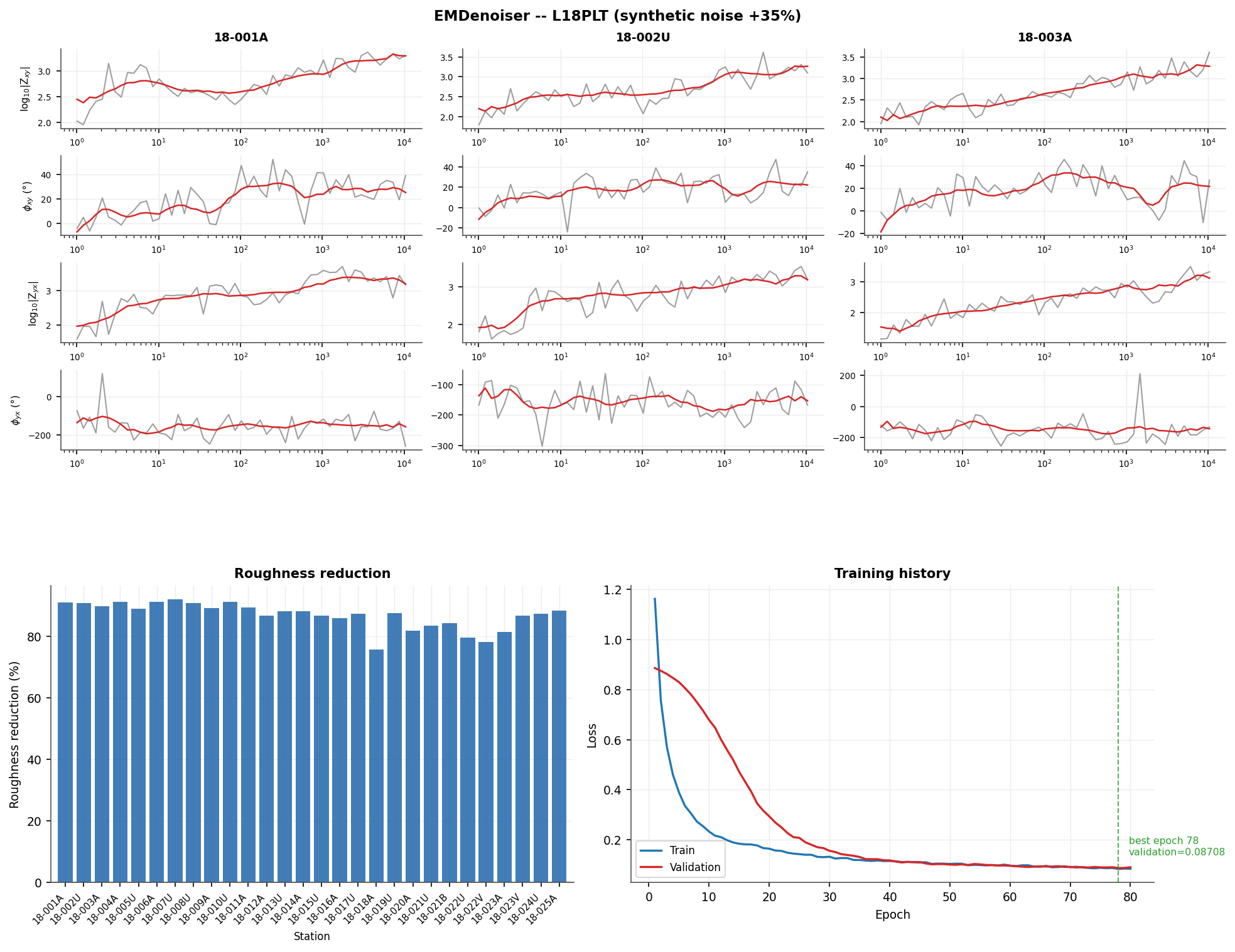
plot_denoise_summary() for three L18PLT stations: before/after spectra on top, per-station roughness reduction and the training curve on the bottom row.

The bottom-left panel plots a unit-free diagnostic instead of RMSE: the percentage reduction in roughness – the mean absolute second difference along the frequency axis, large for a jagged curve and small for a smooth one – from the noisy input to the denoised output. Every station improves by 76-92%, meaning the network suppressed high-frequency scatter fairly uniformly across the whole line rather than helping only a handful of easy stations, consistent with the per-channel RMSE breakdown above once \(\phi_{yx}\)’s wrap issue is set aside. The training curve (bottom-right) is produced by plot_training_history(), which every network-based estimator in this package supports through its history_ property:

>>> from pycsamt.ai.processing.plot import plot_training_history
>>> plot_training_history(den, title="EMDenoiser training")

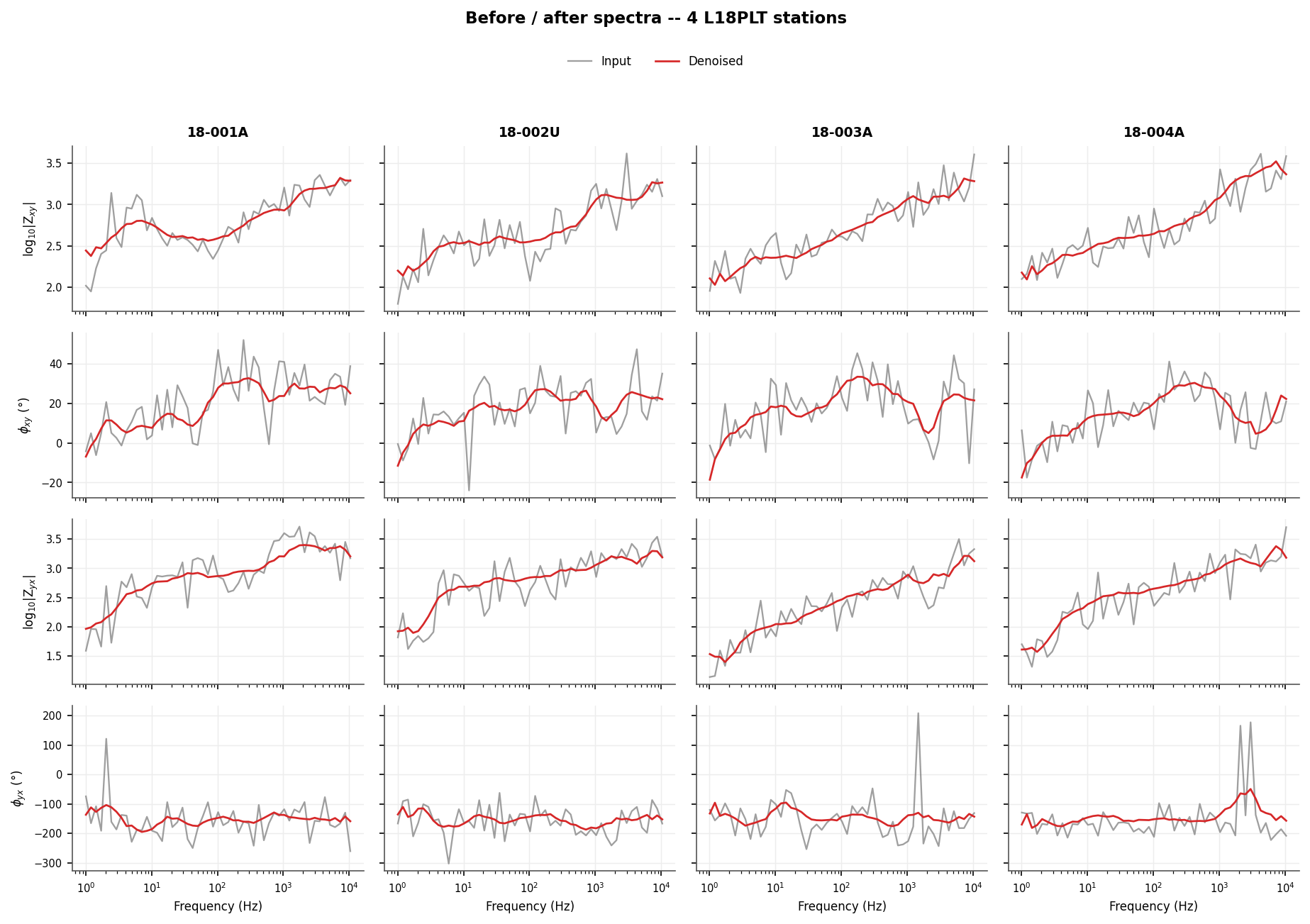
plot_denoise_spectra() at full resolution for four stations – one column per station, one row per feature component. The red denoised curve tracks the smooth trend of the grey input while damping point-to-point spikes, most visibly in the noisy \(\phi_{yx}\) row.

11.27.3.2. Sites in, corrected sites out

Everything above works on the plain (n_sites, n_components, n_freqs) array. For everyday use, apply() skips that array bookkeeping and follows the same sites-in / sites-out convention as the rule-based correction functions in Noise Removal And Spatial Filtering (for example notch_powerline()): pass a site collection, get a corrected one back, with an inplace flag controlling whether the input is mutated or left untouched.

>>> clean_sites = den.apply(sites, inplace=False)
>>> type(clean_sites).__name__
'Sites'

The returned collection has the same station count and the same per-station frequency grid as the input – only Z.z changes, and only in the components the network models:

>>> import numpy as np
>>> from pycsamt.emtools._core import _get_z_block, _iter_items
>>> ed_in = next(_iter_items(sites))
>>> ed_out = next(_iter_items(clean_sites))
>>> _, z_in, _ = _get_z_block(ed_in, with_errors=False)[:3]
>>> _, z_out, _ = _get_z_block(ed_out, with_errors=False)[:3]
>>> z_in.shape == z_out.shape
True
>>> bool(np.allclose(z_in[:, 0, 1], z_out[:, 0, 1]))   # Zxy: denoised
False
>>> bool(np.allclose(z_in[:, 0, 0], z_out[:, 0, 0]))   # Zxx: untouched
True

clean_sites can then feed straight into the next step of a processing chain – another rule-based emtools correction, an inversion input builder, or Pipeline System – exactly the way a plain rule-based correction function’s output would.

Warning

freq_ref (default: the first site’s own grid, matching prepare_z_features()’s own default) must resolve to the same grid used when the training features were built. Calling apply() on the exact collection used for training, or on a collection sharing its first station, reproduces that grid automatically; pass freq_ref explicitly whenever that is not the case.

11.27.3.3. Parameters and limitations

channels sets the encoder/decoder width at each stage (default (64, 128, 64), narrowed to (32, 64, 32) above for a 28-station training set); a wider network has more capacity to overfit a small survey, so shrink it for small n_sites. noise_level is the standard deviation of the synthetic training corruption, relative to each channel’s own standard deviation – too low and the network barely learns to denoise anything; too high and it can over-smooth genuine structure along with noise. dropout (default 0.1) regularizes the bottleneck.

Note

When neither PyTorch nor TensorFlow is installed, EMDenoiser falls back to a per-channel Gaussian filter (scipy.ndimage.gaussian_filter1d). The interface is identical, but there is no learned component and no history_ to plot – plot_training_history() raises ValueError in that case, exactly as it does for any estimator with an empty training history.

Full signatures: EMDenoiser, prepare_z_features(), plot_denoise_spectra(), plot_denoise_noise_reduction(), plot_denoise_summary(), and plot_training_history().

</>View the complete EMDenoiser example sourceClick to inspect and copy the complete code

def run_denoise(sites, save_dir: Path) -> None:
    print("\n=== EMDenoiser ===")
    freq = None
    X_clean = prepare_z_features(sites, n_components=4)
    labels = station_names(sites)
    print(f"  X_clean shape: {X_clean.shape}")

    rng = np.random.default_rng(0)
    noise = rng.normal(
        scale=0.35 * X_clean.std(axis=(0, 2), keepdims=True),
        size=X_clean.shape,
    ).astype("float32")
    X_noisy = (X_clean + noise).astype("float32")

    den = EMDenoiser(channels=(32, 64, 32))
    den.fit(X_clean, noise_level=0.15, epochs=80, seed=0, verbose=False)
    X_den = den.transform(X_noisy)
    print(f"  {den!r}")
    hist = den.history_
    if hist.get("val_loss"):
        print(f"  final val_loss: {hist['val_loss'][-1]:.5f}")
        print(f"  best val_loss:  {min(hist['val_loss']):.5f}")

    rmse_noisy = float(np.sqrt(np.mean((X_noisy - X_clean) ** 2)))
    rmse_den = float(np.sqrt(np.mean((X_den - X_clean) ** 2)))
    print(f"  RMSE vs. clean reference -- noisy:    {rmse_noisy:.4f}")
    print(f"  RMSE vs. clean reference -- denoised: {rmse_den:.4f}")
    for name, ci in [
        ("log|Zxy|", 0), ("phase_xy", 1), ("log|Zyx|", 2), ("phase_yx", 3),
    ]:
        rn = float(np.sqrt(np.mean((X_noisy[:, ci] - X_clean[:, ci]) ** 2)))
        rd = float(np.sqrt(np.mean((X_den[:, ci] - X_clean[:, ci]) ** 2)))
        print(f"    {name:>9s}: RMSE noisy={rn:.3f} denoised={rd:.3f}")

    from pycsamt.ai.processing.plot import _roughness
    r_noisy = _roughness(X_noisy)
    r_den = _roughness(X_den)
    pct = 100.0 * (r_noisy - r_den) / (r_noisy + 1e-24)
    pct_site = np.nanmedian(pct, axis=1)
    print(f"  roughness reduction per station: "
          f"min={pct_site.min():.1f}% max={pct_site.max():.1f}%")

    # frequency grid: reuse the site's own grid (first site) for the x-axis
    from pycsamt.emtools._core import _get_z_block, _iter_items

    for ed in _iter_items(sites):
        result = _get_z_block(ed, with_errors=False)
        freq = result[2] if len(result) >= 3 else None
        if freq is not None:
            break

    fig = plot_denoise_summary(
        freq, X_noisy, X_den, history=den, station_labels=labels,
        n_show=3, suptitle="EMDenoiser -- L18PLT (synthetic noise +35%)",
    )
    _save(fig, save_dir, "denoise_summary.png")

    fig = plot_denoise_spectra(
        freq, X_noisy, X_den, station_labels=labels, n_show=4,
        suptitle="Before / after spectra -- 4 L18PLT stations",
    )
    _save(fig, save_dir, "denoise_spectra.png")

Point load_l18() at your own EDI folder to adapt this script