
18.22. Run a Pipeline From Config#
This tutorial shows how to run a reproducible pyCSAMT processing pipeline from a configuration file. The workflow is designed for survey processing that must be repeated, reviewed, shared, or used as evidence before inversion.
The central idea is:
put the processing chain in a small config file, run that config from Python or the CLI, and let pyCSAMT write the processed EDIs, plots, reports, and a copy of the pipeline that was actually executed.
18.22.1. What You Will Learn#
After this tutorial you should be able to:
create a YAML pipeline configuration file
understand the
name,output_dir,preset, andstepskeysload a pipeline with
pycsamt.pipeline.Pipeline.from_yaml()inspect the resolved processing chain before running it
run the pipeline on an EDI survey
control processed EDI, plot, and report outputs
debug a pipeline with
--dry-run,--n-steps,--from-step, and--until-stepread the returned
PipelineResultuse the equivalent
pycsamt pipeCLI commandspick a method-aware preset (
mt_qc,amt_qc,csamt_qc,csumt_qc) instead of hand-writing frequency-band overridesresume an interrupted run with the step step cache
watch live per-step progress and query the run history log
generate the branded dashboard report alongside the plain one
18.22.2. Why Use a Config File?#
Interactive notebooks are useful for exploration, but production survey processing needs a stronger record. A config file makes the processing chain explicit:
the ordered step list is visible;
every parameter override is written down;
the same file can be used from Python and the CLI;
a colleague can review the workflow before it is run;
output reports can point back to the exact pipeline file;
the same workflow can be applied to several lines or surveys.
For quick experiments, a preset such as Pipeline.from_preset("basic_qc") is
fine. For project work, write the workflow to YAML.
18.22.3. Input Assumptions#
The examples below assume:
EDI files are stored in
data/AMT/WILLY_DATA/L18PLT;the pipeline config will be stored at
config/l18_first_qc.yaml;output will be written to
results/l18_first_qc.
The bundled L18PLT line is a flat EDI folder:
data/
  AMT/
    WILLY_DATA/
      L18PLT/
        18-001A.edi
        18-002U.edi
        ...
        18-025A.edi
If your survey has several independent lines, start by running the workflow on one line. After the parameters are stable, apply the same config to the other lines.
18.22.4. Create a Minimal YAML Config#
This is a complete first-pass QC pipeline:
 1name: l18_first_qc
 2output_dir: results/l18_first_qc
 3
 4steps:
 5  - name: notch
 6    code: NR001
 7    params:
 8      mains_hz: 50.0
 9      n_harm: 30
10      tol_hz: 0.08
11
12  - name: drop_duplicates
13    code: FREQ002
14
15  - name: select_band
16    code: FREQ001
17    params:
18      band_hz: [1.0, 10000.0]
19
20  - name: align_grid
21    code: FREQ004
22
23  - name: qc_snapshot
24    code: QC001
Save it as config/l18_first_qc.yaml.
The keys mean:
nameHuman-readable label used in summaries and reports.
output_dirDefault output directory when
Pipeline.runis called without an explicitoutdir.stepsOrdered processing operations. Each item is converted to a
pycsamt.pipeline.Step.nameinside a stepUser label for that occurrence of the step. This label appears in output folders and can be used for partial runs.
codeRegistry code, such as
NR001orFREQ001. Registry names such asnotch_powerlinecan also be used, but codes are easier to audit.paramsKeyword arguments forwarded to the underlying processing function. Values here override the step defaults.
NR001’smains_hzalso accepts the literal string"auto"to detect 50 vs 60 Hz from the survey’s own frequency grid instead of assuming an exact value – see Pipeline Steps.
The configured chain is intentionally short: remove harmonic power-line noise, normalise the frequency rows, keep the survey band used for this first QC pass, align the station grids, and then write a diagnostic snapshot.
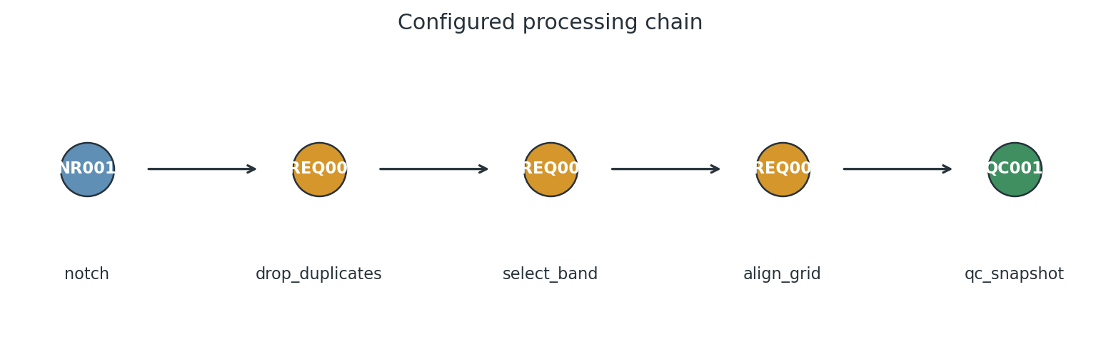
Five explicit steps are easier to review than a long automatic workflow.#
18.22.5. Load and Inspect the Pipeline#
Load the YAML file with pycsamt.pipeline.Pipeline.from_yaml():
 1>>> from pycsamt.pipeline import Pipeline
 2>>> pipe = Pipeline.from_yaml("config/l18_first_qc.yaml")
 3>>> print(pipe)
 4Pipeline  'l18_first_qc'  ───────────────────────────────────────────────  5 steps
 5  ( 1) notch            [NR001]    Power-line Harmonic Notch   mains_hz=50.0  n_harm=30  tol_hz=0.08
 6  ( 2) drop_duplicates  [FREQ002]  Drop Duplicate Frequencies
 7  ( 3) select_band      [FREQ001]  Frequency Band Select       band_hz=[1.0, 10000.0]
 8  ( 4) align_grid       [FREQ004]  Frequency Grid Alignment
 9  ( 5) qc_snapshot      [QC001]    QC Quick-Look Snapshot
10────────────────────────────────────────────────────────────────────────────────
For a dataframe view of the resolved steps:
1>>> table = pipe.describe()
2>>> print(table[["label", "code", "category", "params"]])
3             label     code       category                                            params
4#
51            notch    NR001  noise_removal  {'mains_hz': 50.0, 'n_harm': 30, 'tol_hz': 0.08}
62  drop_duplicates  FREQ002      frequency                                                {}
73      select_band  FREQ001      frequency                       {'band_hz': [1.0, 10000.0]}
84       align_grid  FREQ004      frequency                                                {}
95      qc_snapshot    QC001             qc                                                {}
Before running a workflow for the first time, inspect the steps and check:
the order matches the processing logic;
labels are unique and readable;
frequency limits match the survey type;
power-line settings match the local electrical grid;
diagnostic steps such as
QC001appear where you want snapshots.
18.22.6. Read the Survey#
Read the EDI survey through the public API:
 1>>> from pycsamt.api import read_edis
 2>>> survey = read_edis(
 3...     "data/AMT/WILLY_DATA/L18PLT",
 4...     recursive=False,
 5...     strict=False,
 6...     progress=False,
 7... )
 8>>> sites = survey.collection
 9>>> print(survey.summary())
10APIFrame: edi_survey_summary
11kind: edi.summary
12shape: 28 rows x 6 columns
13columns: station, path, n_freq, tipper, spectra, ts
14numeric: 1 columns
15missing: 0.0%
16source: data/AMT/WILLY_DATA/L18PLT
The pipeline runs on a site collection. survey.collection is the lower-level
object used by the pipeline and by the editing/QC tools. The bundled line loads
as 28 stations.
18.22.7. Run the Pipeline#
Run the loaded pipeline:
1>>> result = pipe.run(sites)
2>>> print(result.summary())
Because the config defines output_dir, this writes to
results/l18_first_qc. To override the output directory from Python:
1>>> result = pipe.run(
2...     sites,
3...     outdir="results/l18_first_qc_trial_02",
4... )
To run fully in memory with no filesystem output:
1>>> result = pipe.run(
2...     sites,
3...     outdir=None,
4...     save_plots=False,
5...     save_edis=False,
6...     save_report=False,
7... )
18.22.8. Inspect the Result#
Pipeline.run returns a PipelineResult:
1>>> print(result.ok)
2True
3>>> print(result.n_errors)
40
5>>> print(result.outdir)
6results/l18_first_qc
7>>> processed_sites = result.sites_out
Each step also has a StepResult:
1>>> for step_result in result.step_results:
2...     print(step_result.summary_line())
3...
4>>> failed = [sr for sr in result.step_results if not sr.ok]
5>>> for sr in failed:
6...     print(sr.step_name, sr.step_code, sr.error)
By default, the pipeline continues after step errors according to the pipeline
runtime configuration. For strict production runs, configure the error policy
or use the CLI --on-error raise option.
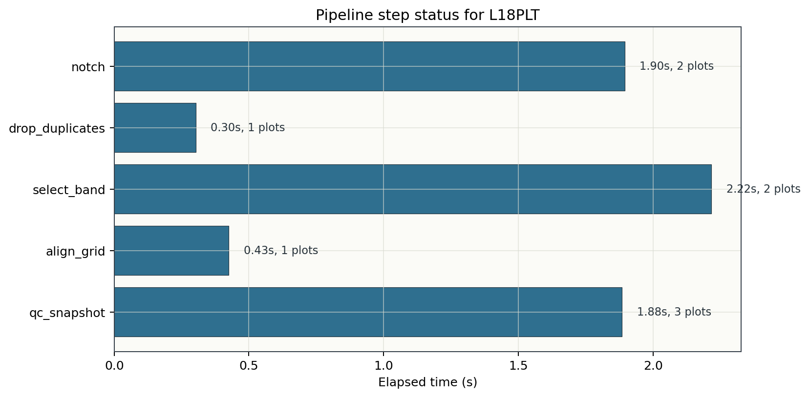
For the bundled L18PLT line, the full run completes with all five steps OK:
PipelineResult  'l18_first_qc'
  Sites   : 28 in → 28 out
  Steps   : 5 (5 ok, 0 err)
  Time    : 23.94 s
  Plots   : 9
  Output  : results/l18_first_qc

[ 1] notch                [NR001]  OK  3.60s  sites 28→28  plots=2
[ 2] drop_duplicates      [FREQ002]  OK  1.12s  sites 28→28  plots=1
[ 3] select_band          [FREQ001]  OK  8.67s  sites 28→28  plots=2
[ 4] align_grid           [FREQ004]  OK  1.50s  sites 28→28  plots=1
[ 5] qc_snapshot          [QC001]  OK  9.81s  sites 28→28  plots=3
Timings vary by machine, but the station count, step status, and artifact counts are the values to check first.
18.22.9. Understand the Output Folder#
A normal run writes a directory like this:
results/l18_first_qc/
  pipeline.yaml
  plots/
    01_notch/
      nr_qc_harmonic_waterfall.png
      nr_qc_snr_gain_profile.png
    02_drop_duplicates/
      plot_coverage_quality_heatmap.png
    03_select_band/
      plot_band_microstrips.png
      plot_coverage_quality_heatmap.png
    04_align_grid/
      plot_coverage_quality_heatmap.png
    05_qc_snapshot/
      plot_coverage_psection.png
      plot_qc_quicklook.png
      plot_station_confidence_dashboard.png
  processed/
    18-001A.edi
    18-002U.edi
    ...
  report.html
  summary.txt
The important files are:
processed/Final processed EDI files written after the last step.
plots/Per-step QC figures generated by the step registry.
pipeline.yamlCanonical copy of the pipeline that was run. Keep this with the output.
summary.txtText run report for quick inspection.
report.htmlHTML run report for project records and review.
The output tree is intentionally stable so that scripts, reports, and later inversion preparation can point to predictable paths.
The example run writes 28 processed EDI files, 9 QC figures, 2 reports, and 1 saved copy of the pipeline config:
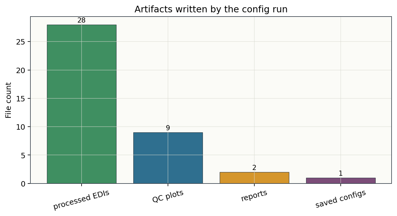
report.html and summary.txt are written by default. A third,
opt-in dashboard report (dashboard.html) with KPI stat tiles
and charts is added alongside them when requested – see Beyond the
Basics below.
18.22.10. Generate a Starter Config#
The CLI can scaffold a valid config:
1pycsamt pipe init \
2    --preset basic_qc \
3    --name l18_first_qc \
4    --outdir results/l18_first_qc \
5    --output config/l18_first_qc.yaml
Print a scaffold without writing it:
1pycsamt pipe init --preset full_processing --print
Generate JSON or Python config files when needed:
1pycsamt pipe init --format json --preset basic_qc -o config/l18_first_qc.json
2pycsamt pipe init --format py --preset basic_qc -o config/l18_first_qc.py
YAML is recommended for most survey projects. Python configs are useful for trusted internal workflows that need constants or small local logic.
18.22.11. Seed a Config From a Preset#
You can combine a preset with explicit steps. Preset steps run first, and the steps listed in the file are appended afterward:
1name: publication_with_extra_qc
2output_dir: results/publication_with_extra_qc
3preset: publication_ready
4
5steps:
6  - name: final_qc
7    code: QC001
This is useful when a built-in preset is almost correct but you want one or two
additional operations. If you need to remove or reorder many preset steps, copy
the preset into an explicit steps list instead. Explicit files are easier
to review.
18.22.12. Discover Steps and Presets#
From Python:
 1>>> from pycsamt.pipeline import Pipeline, list_steps, preset_catalogue
 2>>> for spec in list_steps("frequency"):
 3...     print(spec.code, spec.name, spec.defaults)
 4...
 5FREQ001 select_band {'band_hz': (0.001, 10000.0)}
 6FREQ002 drop_duplicates {}
 7FREQ003 drop_low_confidence {}
 8FREQ004 align_grid {}
 9FREQ005 regrid_logspace {'n_per_decade': 6}
10FREQ006 decimate {'step': 2}
11FREQ007 smooth_freq {'window': 3}
12FREQ008 mask_low_confidence {'method': 'composite', 'threshold': 0.5}
13FREQ009 recover_low_confidence {'method': 'composite', 'ci_hi': 0.9, 'ci_lo': 0.5, 'interpolation': 'linear'}
14>>> print(Pipeline.step_info("NR001"))
15────────────────────────────────────────────────────────────────────
16  NR001  Power-line Harmonic Notch  [noise_removal]
17────────────────────────────────────────────────────────────────────
18  name     : notch_powerline
19  function : pycsamt.emtools.remove_noise.notch_powerline
20  defaults : mains_hz=50  n_harm=30  tol_hz=0.08
21  qc plots : nr_qc_harmonic_waterfall, nr_qc_snr_gain_profile
22  returns  : Sites (transform)
23────────────────────────────────────────────────────────────────────
preset_catalogue() prints every registered preset, including the four
method-aware ones, with its description and step sequence.
From the CLI:
1pycsamt pipe presets
2pycsamt pipe steps
3pycsamt pipe steps --category frequency
4pycsamt pipe show --preset publication_ready
Use discovery before editing a config so you know the registered code, default parameters, and category for each operation.
18.22.13. Run From the CLI#
Run the same YAML file from the command line:
1pycsamt pipe run \
2    --config config/l18_first_qc.yaml \
3    --survey data/AMT/WILLY_DATA/L18PLT \
4    --out results/l18_first_qc
The positional source form is also accepted:
1pycsamt pipe run data/AMT/WILLY_DATA/L18PLT --config config/l18_first_qc.yaml --out results/l18_first_qc
Use verbose mode to show progress:
1pycsamt pipe run \
2    --config config/l18_first_qc.yaml \
3    --survey data/AMT/WILLY_DATA/L18PLT \
4    --out results/l18_first_qc \
5    -v
Useful output controls:
1pycsamt pipe run --config config/l18_first_qc.yaml --survey data/AMT/WILLY_DATA/L18PLT --no-plots
2pycsamt pipe run --config config/l18_first_qc.yaml --survey data/AMT/WILLY_DATA/L18PLT --no-edi
3pycsamt pipe run --config config/l18_first_qc.yaml --survey data/AMT/WILLY_DATA/L18PLT --no-report
4pycsamt pipe run --config config/l18_first_qc.yaml --survey data/AMT/WILLY_DATA/L18PLT --plot-fmt pdf --dpi 300
Use machine-readable output for automation:
1pycsamt pipe run \
2    --config config/l18_first_qc.yaml \
3    --survey data/AMT/WILLY_DATA/L18PLT \
4    --format json
18.22.14. Debug Before Running#
Always dry-run a new config:
1pycsamt pipe run \
2    --config config/l18_first_qc.yaml \
3    --survey data/AMT/WILLY_DATA/L18PLT \
4    --dry-run
Preview the pipeline table:
1pycsamt pipe show config/l18_first_qc.yaml
2pycsamt pipe show config/l18_first_qc.yaml --format json
Run only the first steps:
1pycsamt pipe run \
2    --config config/l18_first_qc.yaml \
3    --survey data/AMT/WILLY_DATA/L18PLT \
4    --n-steps 2 \
5    --out results/debug_first_two
Start or stop at a named step:
 1pycsamt pipe run \
 2    --config config/l18_first_qc.yaml \
 3    --survey data/AMT/WILLY_DATA/L18PLT \
 4    --from-step select_band \
 5    --out results/debug_from_band
 6
 7pycsamt pipe run \
 8    --config config/l18_first_qc.yaml \
 9    --survey data/AMT/WILLY_DATA/L18PLT \
10    --until-step align_grid \
11    --out results/debug_until_align
The slicing options accept the user step label, the registry code, or the
registry name. For example, select_band, FREQ001, and the internal
step name can all identify the same operation when present in the pipeline.
18.22.15. Error Policy#
During exploratory work, it is often useful to continue after a step fails so you can see how much of the pipeline still works. During production work, fail fast.
CLI options:
1pycsamt pipe run --config config/l18_first_qc.yaml --survey data/AMT/WILLY_DATA/L18PLT --on-error warn
2pycsamt pipe run --config config/l18_first_qc.yaml --survey data/AMT/WILLY_DATA/L18PLT --on-error skip
3pycsamt pipe run --config config/l18_first_qc.yaml --survey data/AMT/WILLY_DATA/L18PLT --on-error raise
Python configuration:
1>>> from pycsamt.pipeline import configure_pipe
2>>> configure_pipe(on_step_error="raise")
3>>> result = pipe.run(sites, outdir="results/strict_run")
Use raise for final processing before inversion or publication output.
18.22.16. Choose a Method-Aware Preset#
The config above is intentionally generic – it treats every survey the same
way. In reality MT, AMT, CSAMT, and CSUMT are not interchangeable: CSAMT and
CSUMT use a controlled source and can suffer near-field/transition-zone
contamination that MT and AMT never see, a single-component TE- or TM-only
CSAMT line cannot produce a meaningful phase-tensor ellipse, and tipper is
only sometimes recorded at all. mt_qc, amt_qc, csamt_qc, and
csumt_qc are four built-in presets that account for this: each still
denoises and cleans frequencies the way basic_qc does, but adds the
correction and diagnostics appropriate to its method, and every QC plot
checks the actual data before deciding whether to draw itself, instead of
always producing the same figures regardless of what the survey contains. See
Pipeline Presets’s “Method-Aware Presets” section for the
full mechanism; this section shows the parts a user actually touches.
Pick a preset by method name rather than memorising which one is which:
1>>> from pycsamt.pipeline import get_preset_for_method
2>>> get_preset_for_method("AMT").name
3'amt_qc'
4>>> get_preset_for_method("CSAMT").name
5'csamt_qc'
Running amt_qc against the same L18PLT survey used throughout this
tutorial shows what it adds over the plain config above: a raw-data preview,
strike analysis, and data-driven phase-tensor/tipper QC, opening and closing
with a preview of the same randomly (but deterministically) chosen stations
before and after processing:
 1>>> from pycsamt.pipeline import Pipeline
 2>>> pipe = Pipeline.from_preset("amt_qc")
 3>>> print(pipe)
 4Pipeline  'amt_qc'  ────────────────────────────────────────────────────  11 steps
 5  ( 1) raw_preview        [PRE001]   Raw Data Preview (random stations)
 6  ( 2) notch              [NR001]    Power-line Harmonic Notch                 mains_hz=50  n_harm=30  tol_hz=0.08
 7  ( 3) drop_dup           [FREQ002]  Drop Duplicate Frequencies
 8  ( 4) select_band        [FREQ001]  Frequency Band Select                     band_hz=(10.0, 100000.0)
 9  ( 5) align_grid         [FREQ004]  Frequency Grid Alignment
10  ( 6) rotate_strike      [TZ001]    Strike Rotation                           method='swift'
11  ( 7) qc_snapshot        [QC001]    QC Quick-Look Snapshot
12  ( 8) strike_qc          [QC007]    Strike Analysis & Rose QC
13  ( 9) tensor_qc_smart    [QC005]    Phase Tensor QC (multi-component only)
14  (10) tipper_qc_smart    [QC006]    Tipper QC (tipper-present only)
15  (11) processed_preview  [PRE002]   Processed Data Preview (random stations)
16────────────────────────────────────────────────────────────────────────────────
17>>> result = pipe.run(sites, outdir="results/l18_amt_qc", save_edis=False)
18>>> print(result.summary())
19PipelineResult  'amt_qc'
20  Sites   : 28 in → 28 out
21  Steps   : 11 (11 ok, 0 err)
22  Time    : 72.37 s
23  Plots   : 16
QC005 (phase-tensor QC) fires here because L18PLT is full-tensor data
– phase_tensor_smart.png is among the 16 figures. QC006 (tipper QC)
runs too, but produces nothing: L18PLT, like most AMT lines, carries no
tipper channel, so all five tipper-dependent plots are silently skipped
rather than drawn empty. Nothing needed to be configured for either of these
outcomes – the gating reads the data itself.
Near-field correction, by contrast, genuinely needs a controlled-source
survey to demonstrate – AMT data has no source to correct for. Running
csamt_qc against the real 10-station Tongkeng CSAMT line bundled at
data/CSAMT (see [Kouadio2020] in References) shows the
other half of what a method-aware preset adds:
1>>> survey = read_edis("data/CSAMT", recursive=False, strict=False, progress=False)
2>>> pipe = Pipeline.from_preset("csamt_qc")
3>>> result = pipe.run(survey.collection, outdir="results/csamt_qc")
4>>> print(result.summary())
5PipelineResult  'csamt_qc'
6  Sites   : 10 in → 10 out
7  Steps   : 14 (14 ok, 0 err)
8  Time    : 50.12 s
9  Plots   : 17
A UserWarning is raised once per station along the way:
correct_near_field: no source offset for 'csa000'; station skipped.
correct_near_field: no source offset for 'csa050'; station skipped.
correct_near_field: no source offset for 'csa100'; station skipped.
...
This is expected, not a bug: csamt_qc’s near-field-correction step
(SRC001) runs with source_offset=None, meaning “resolve the real
transmitter-receiver separation from each station’s own metadata, and warn
instead of failing when nothing resolves.” This particular bundled dataset’s
EDI headers don’t carry that offset, so every station passes through
uncorrected – result.ok is still True. When a survey’s offset is
available (passed explicitly, or present as source_offset/
offset/dist on the site metadata), the correction is real: it divides
the impedance tensor by the complex near-field factor
\(F(p) = 1 - 3/p^2 + 3/p^3\), not a no-op.
QC002 (field_zone_snapshot) plots the near/transition/far-field
classification regardless of whether the correction itself could run, using
whatever offset is available. Supplying an illustrative 2000 m offset
directly to pycsamt.emtools.fieldzone.plot_field_zones() – a stand-in
since this dataset’s own headers don’t carry the real transmitter geometry
– shows the pattern a real corrected survey’s pseudosection looks like:
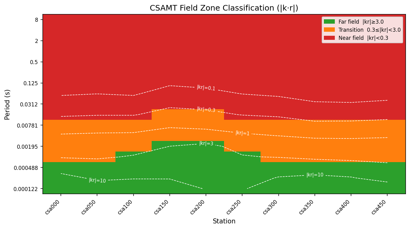
Red marks the near field (|k·r| < 0.3), orange the transition
zone, and green the far field where the plane-wave approximation holds.
The near-field band widens toward the low-frequency (long-period) end of
the sounding, which is the classic CSAMT symptom near-field
correction exists to address: at long periods the receiver sits too
close to the source, relative to skin depth, for the plane-wave
assumption behind standard MT/AMT processing to hold.#
csumt_qc follows the same pattern as csamt_qc – near-field
correction, the same zone pseudosection – trimmed to the real CSUMT
acquisition band (9.6 kHz - 614.4 kHz) and with an added Bostick
depth-section snapshot; see Pipeline Presets for its
exact step sequence.
18.22.17. Beyond the Basics#
Four more opt-in capabilities matter once a config graduates from “quick
check” to “something a project relies on.” None of them change how a
pipeline processes data or affect a run that doesn’t ask for them; each is
covered in full depth on its own page, linked below. Combined on the same
l18_first_qc.yaml config:
1pycsamt pipe run \
2    --config config/l18_first_qc.yaml \
3    --survey data/AMT/WILLY_DATA/L18PLT \
4    --out results/l18_first_qc \
5    --cache --history --dashboard \
6    -v
--cacheKeys each step’s output by the exact upstream data, step code, and parameters. A crashed or interrupted run resumes for free: rerunning the identical command replays every already-completed step from the step cache instead of recomputing it. Full mechanism, what is and isn’t safe to cache, and a measured before/after timing comparison (isolated from figure generation) in Caching And Resume.
--liveReplaces the static progress bar with a live-updating status table (pending/running/OK/ERR/cached, one row per step, rewritten in place). Full rendering example in Live Observability.
--historyAppends a one-line JSON summary of the run to a run history log (default
~/.pycsamt/pipeline_history.jsonl), queryable afterward:1pycsamt pipe history --last 2
1Logged 2 pipeline run(s):
2  2026-08-14T15:03:30Z  l18_first_qc         OK               20.38s  sites 28→28
3  2026-08-14T15:04:44Z  l18_first_qc         OK               22.41s  sites 28→28
--dashboardAdds a richer, branded dashboard report (
dashboard.html) alongside the defaultreport.html/summary.txt– KPI stat tiles and inline-SVG charts (step status, per-step duration, site-count flow) built from the same per-step data. Full contents in Pipeline Outputs’s “Dashboard Report” section.
Running the command above once, then again unchanged, replays every step
from cache – the second run’s --format json output shows
"cached": true on all five steps. Total wall time does not collapse to
near-zero in this particular comparison, because QC-figure generation
(the same 9 plots feeding report.html and dashboard.html) is not
itself cache-aware and still runs on every invocation – only the step
transform is skipped. Caching And Resume’s own
captured example isolates this with --no-plots to show the real
transform-only speed-up; in ordinary use, the practical win is resuming a
long or interrupted run without recomputing what already succeeded, not a
faster wall clock on an already-fast five-step config.
18.22.18. Common Workflow Pattern#
A robust project workflow usually looks like this:
Read the survey and build a station inventory.
Run a small config with
notch,drop_duplicates,select_band, andqc_snapshot, or the method-aware*_qcpreset that matches the survey (mt_qc/amt_qc/csamt_qc/csumt_qc).Inspect the generated plots and
summary.txt.Tighten the frequency band or noise parameters.
Add static-shift, tensor, skew, or dimensionality steps only after the first QC pass is understood.
Turn on
--cacheand--historyonce a config stabilises, so later iterations resume instead of recomputing and every run is logged.Save the final config next to the processed output.
Use the processed EDI folder for inversion preparation.
This keeps the processing chain explainable. A short, reviewed config is often better than a long automatic workflow that nobody can defend.
18.22.19. Troubleshooting#
- The config loads but has no steps
Check that the top-level
stepskey is a list. If you used onlypreset, verify the preset name withpycsamt pipe presets.- The CLI says the pipeline cannot be loaded
Confirm the file suffix is
.yaml,.yml,.json, or.py. YAML loading also requiresPyYAML.- The run reports zero sites
Check the
--surveypath or positional EDI path. If EDIs are inside nested line folders, verify that the survey resolver can find them, or load one line directory explicitly first.- The output directory is not the one expected
--outandPipeline.run(outdir=...)overrideoutput_dirin the config. When no explicit output is given, the config value is used, then the global pipeline default.- Processed EDI files are missing
Check whether
--no-ediorsave_edis=Falsewas used. Also review warnings frompycsamt.site.export.write_sitesif the site objects cannot be exported.- Plots are missing
Some steps do not define QC plot functions, and plot generation can be disabled with
--no-plotsorsave_plots=False. Plot failures should not stop a successful processing run.- A step fails but the pipeline continues
This is controlled by the error policy. Use
--on-error raiseorconfigure_pipe(on_step_error="raise")for strict runs.- Near-field correction warns for every station
Expected, not a bug, when a survey’s EDI headers carry no resolvable
source_offset/offset/dist.csamt_qc/csumt_qcruncorrect_near_fieldwithsource_offset=Noneprecisely so this warns and passes the station through uncorrected instead of failing the run. Pass a real offset (a float, or a{station: offset}dict) explicitly if you have one.dashboard.htmlis missingIt is opt-in. Pass
--dashboardon the CLI, or add"dashboard"toreport_formatsin Python – see Beyond the Basics.
18.22.20. Next Steps#
Inspect and QC the input survey with Inspect and QC a Survey.
Correct static shift with Correct Static Shift.
Prepare processed EDIs for Occam2D with Prepare an Occam2D Inversion.
18.22.21. See Also#
- Pipeline Configuration Files
Full configuration-file schema.
- Pipeline Steps
Registered pipeline steps and categories.
- Pipeline Presets
Every built-in preset, including the method-aware
mt_qc/amt_qc/csamt_qc/csumt_qcgroup and the “smart” QC/preview steps behind them.- Caching And Resume
The step cache in full: what is and isn’t safe to cache, and how a crashed run resumes.
- Live Observability
Live progress, the
on_stephook, notebook rendering, and the run history log in full.- Pipeline Outputs
Output directory structure and reports, including the dashboard report.
- Pipeline Commands
Pipeline CLI reference.
- pycsamt.pipeline
Pipeline API reference.