11.19. Phased-Array Source Design

pycsamt.emtools.source_array is the transmitter-design module in emtools. Unlike most pages in this section, it does not load EDI files or operate on Sites objects. It implements formulas for a phased-array source (PAS): a line of controlled-source audio-frequency magnetotelluric dipoles whose relative phases can steer and narrow the transmitted beam.

The traditional source is a single-dipole antenna source, abbreviated SDAS. The phased-array source combines N co-linear SDAS elements with spacing d and inter-element phase shift beta. The module helps you answer practical design questions:

• What wavelength should be used at CSAMT frequencies?

• How directional is one finite-length dipole?

• How much does an N-element array narrow the beam?

• Which phase shift steers the beam to the area of interest?

• Are there unwanted grating lobes?

• How much SNR gain is expected from coherent arraying?

Full function signatures and parameter defaults are maintained in the API reference. The examples below use the public two-level imports from pycsamt.emtools. Most of this page works parametrically, from a chosen frequency and half-space resistivity, so a design can be explored before a survey exists; the closing section anchors the same functions to a grounded dipole transmitter and real frequency band actually acquired.

11.19.1. Concepts And Angles

The module uses two related angle conventions:

Symbol	Used by	Meaning
theta_deg	sdas_element_pattern	Angle from the dipole axis. 0 and 180 degrees are along the dipole; 90 degrees is broadside.
theta_b_deg	array_factor, pas_pattern, plot_radiation_pattern	Broadside angle. 0 degrees is perpendicular to the array; -90 and +90 degrees are end-fire directions.
theta_m_deg	beam_steer	Desired main-lobe broadside angle.

This distinction matters. The element pattern is written in the dipole axis convention, while the array factor is written in the broadside convention. pas_pattern handles the conversion internally.

11.19.2. Workflow Map

Task	Use this	Output
Compute propagation wavenumber	wavenumber	Earth or free-space wavenumber k in m^-1.
Model one finite SDAS dipole	sdas_element_pattern	Normalized amplitude pattern versus dipole-axis angle.
Model array interference	array_factor	Normalized array factor versus broadside angle.
Combine element and array effects	pas_pattern	Total PAS amplitude pattern.
Steer the main beam	beam_steer	Inter-element phase shift beta in radians.
Check all beam solutions	steering_angles	Target beam and any grating-lobe angles.
Estimate single-source directivity	sdas_directivity	Dimensionless directivity from numerical integration.
Estimate coherent SNR gain	snr_gain_db	Gain in decibels, 20 log10(N).
Plot patterns	plot_radiation_pattern	Polar or Cartesian pattern figure.

11.19.3. Earth Wavenumber

For CSAMT transmitter design, use the effective earth wavenumber when a representative half-space resistivity is known:

\[k_\mathrm{earth} = \sqrt{\frac{\pi f \mu_0}{\rho}}\]

If rho is omitted, wavenumber returns the free-space value 2*pi*f/c. That can be useful as a reference, but it is usually the wrong scale for CSAMT array geometry.

>>> import numpy as np
>>> from pycsamt.emtools import wavenumber
>>> freq = 8.0      # Hz
>>> rho = 300.0     # ohm.m
>>> k_earth = wavenumber(freq, rho=rho)
>>> k_free = wavenumber(freq)
>>> wavelength_earth = 2.0 * np.pi / k_earth
>>> wavelength_free = 2.0 * np.pi / k_free
>>> print(f"earth wavelength: {wavelength_earth:,.0f} m")
earth wavelength: 19,365 m
>>> print(f"free-space wavelength: {wavelength_free:,.0f} m")
free-space wavelength: 37,474,057 m

Use the earth wavelength to judge whether the chosen element spacing is small, moderate, or large in wavelengths:

>>> d = 2000.0
>>> print(f"d / earth wavelength = {d / wavelength_earth:.3f}")
d / earth wavelength = 0.103

A physical spacing that is small at low frequency can become larger than one wavelength at a high CSAMT frequency. That is when side lobes and grating lobes become much more important.

11.19.4. Single-Dipole Element Pattern

sdas_element_pattern computes the finite-length SDAS element pattern:

\[F(\theta) = \left| \frac{\cos(k l \cos\theta / 2) - \cos(k l / 2)} {\sin\theta} \right|\]

Here theta is measured from the dipole axis. Along the dipole axis the response is a null. Broadside to the dipole the normalized response is usually the maximum.

>>> import matplotlib.pyplot as plt
>>> from pycsamt.emtools import sdas_element_pattern, wavenumber
>>> freq = 8.0
>>> rho = 300.0
>>> length = 1000.0
>>> k = wavenumber(freq, rho=rho)
>>> theta = np.linspace(0.0, 180.0, 721)
>>> element = sdas_element_pattern(theta, l=length, k=k)
>>> print(element[0], element[360], element[-1])
0.0 1.0 0.0
>>> fig, ax = plt.subplots(figsize=(7, 4))
>>> _ = ax.plot(theta, element)
>>> _ = ax.set_xlabel("Angle from dipole axis (deg)")
>>> _ = ax.set_ylabel("Normalized amplitude")
>>> _ = ax.grid(True, alpha=0.3)
>>> fig.tight_layout()
>>> fig.savefig("sdas_element_pattern.png", dpi=200)
>>> plt.close(fig)

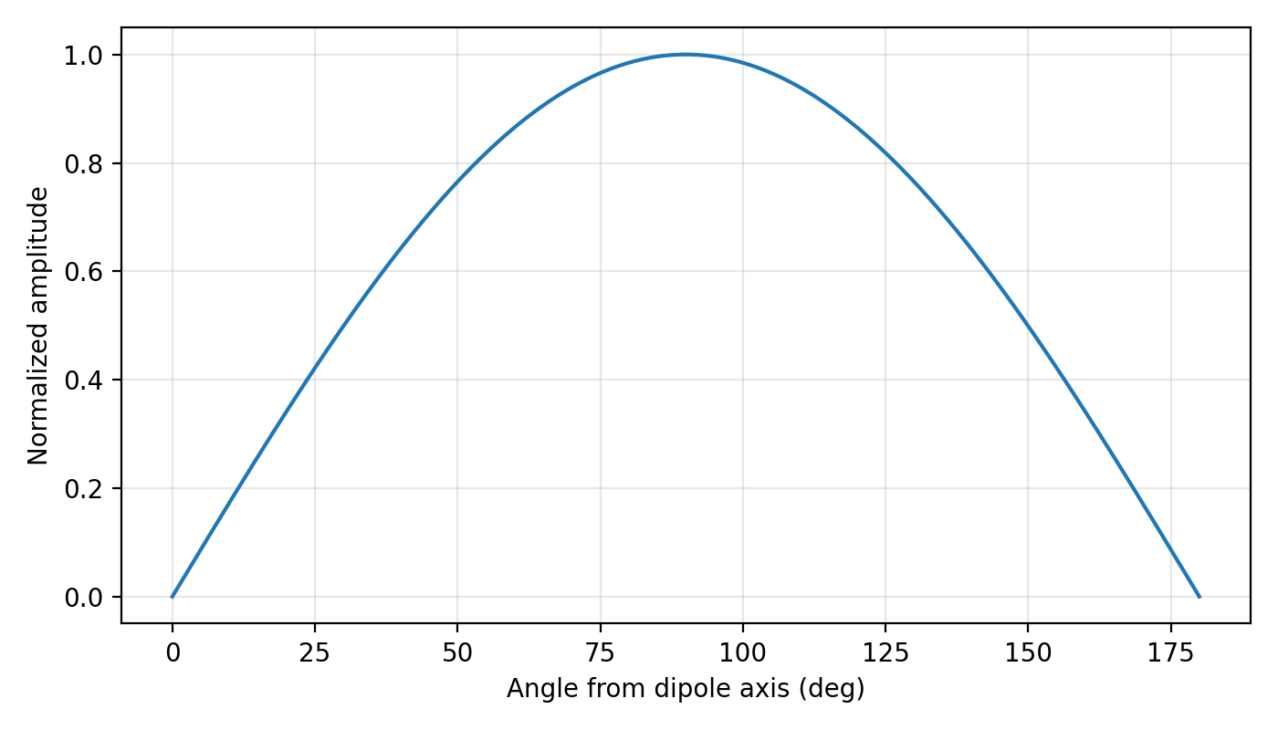
Angle 0 is along the dipole (a null), angle 90 (index 360 on this 721-point grid) is broadside (the normalized peak, 1.0), and angle 180 is the opposite null – exactly the three printed values above. Set normalize=False when you need the unnormalized formula value, for example before computing directivity or comparing absolute pattern shape for different lengths.

11.19.5. Array Factor

array_factor models interference among N equally spaced co-linear source elements. The array factor is the part of the radiation pattern caused by geometry and phase shifts alone:

\[AF_n = \frac{\sin(N \psi / 2)} {N \sin(\psi / 2)}\]

\[\psi = k d \sin(\theta_b) + \beta\]

The angle theta_b is measured from broadside. With beta=0, the main lobe is broadside at theta_b = 0.

>>> from pycsamt.emtools import array_factor, plot_radiation_pattern, wavenumber
>>> freq = 8.0
>>> rho = 300.0
>>> d = 2000.0
>>> k = wavenumber(freq, rho=rho)
>>> theta_b = np.linspace(-90.0, 90.0, 721)
>>> patterns = [
...     array_factor(theta_b, N=1, d=d, k=k),
...     array_factor(theta_b, N=2, d=d, k=k),
...     array_factor(theta_b, N=4, d=d, k=k),
...     array_factor(theta_b, N=8, d=d, k=k),
... ]
>>> ax = plot_radiation_pattern(
...     theta_b,
...     patterns,
...     labels=["N=1", "N=2", "N=4", "N=8"],
...     title="Array factor at 8 Hz",
... )
>>> ax.figure.savefig("array_factor_8hz.png", dpi=200)
>>> plt.close(ax.figure)

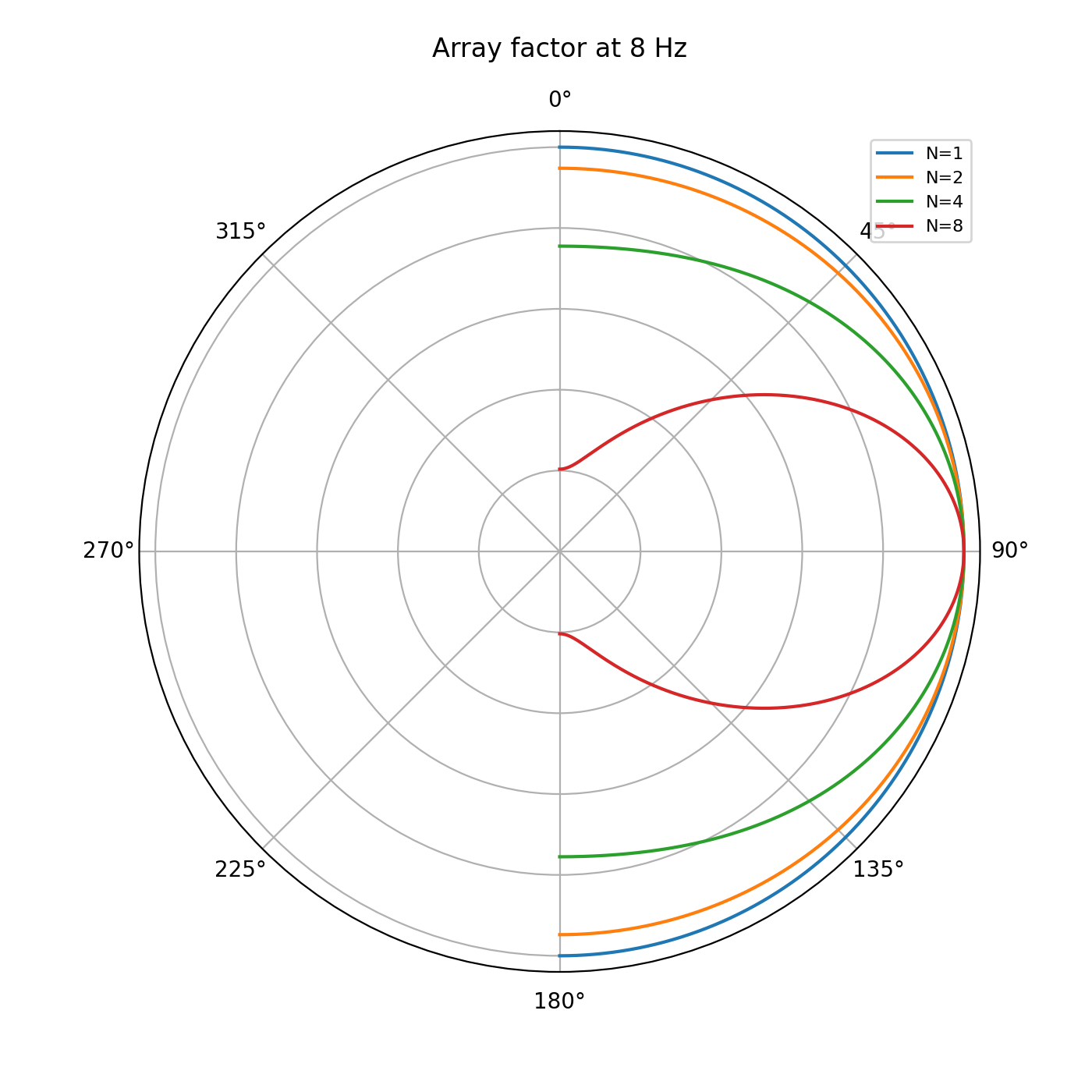
At low frequency, a kilometer-scale array may be much smaller than one earth wavelength – d / earth wavelength was only 0.103 at 8 Hz above. It can still narrow the beam, but it may not form sharp nulls. Recompute the pattern at the high end of the frequency sweep before trusting a design.

11.19.6. High-Frequency Check

The same physical layout can behave very differently at higher frequency.

>>> rho = 300.0
>>> d = 2000.0
>>> freq = 1024.0
>>> k = wavenumber(freq, rho=rho)
>>> wavelength = 2.0 * np.pi / k
>>> theta_b = np.linspace(-90.0, 90.0, 721)
>>> patterns = [array_factor(theta_b, N=n, d=d, k=k) for n in (1, 2, 4, 8)]
>>> print(f"d / wavelength = {d / wavelength:.3f}")
d / wavelength = 1.168
>>> ax = plot_radiation_pattern(
...     theta_b,
...     patterns,
...     labels=["N=1", "N=2", "N=4", "N=8"],
...     polar=False,
...     log_scale=True,
...     title="Array factor at 1024 Hz",
... )
>>> ax.figure.savefig("array_factor_1024hz.png", dpi=200)
>>> plt.close(ax.figure)

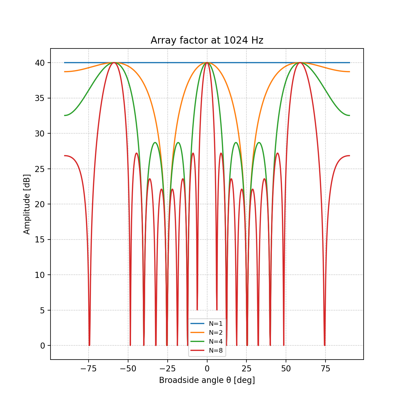
The same 2000 m spacing that was a tenth of a wavelength at 8 Hz is now 1.168 wavelengths at 1024 Hz. When d / wavelength approaches or exceeds 1, grating lobes are likely. A design that looks clean at low frequency can radiate strongly in unintended directions at high frequency.

11.19.7. Beam Steering

beam_steer computes the inter-element phase shift required to steer the main lobe:

\[\beta = -k d \sin(\theta_m)\]

Use steering_angles immediately after beam_steer. The array factor is periodic in \(\psi\), so the same main-lobe condition \(\psi = kd\sin\theta_b+\beta = 0\) that fixes the target angle is also satisfied whenever \(\psi\) is any other multiple of \(2\pi\):

\[kd\sin\theta_n + \beta = 2\pi n, \qquad n = 0, \pm1, \pm2, \dots, \qquad \theta_n = \arcsin\!\left(\frac{2\pi n - \beta}{kd}\right),\]

keeping only the integers \(n\) for which the argument of \(\arcsin\) stays in \([-1, 1]\) – a real broadside angle. Every extra solution besides the intended \(\theta_m\) is a grating lobe: a second, equally strong main lobe pointed somewhere you did not design for. steering_angles reveals whether the requested beam has any of these additional solutions.

>>> from pycsamt.emtools import beam_steer, steering_angles
>>> freq = 1024.0
>>> rho = 300.0
>>> d = 2000.0
>>> N = 4
>>> target_angle = 20.0
>>> k = wavenumber(freq, rho=rho)
>>> beta = beam_steer(target_angle, d=d, k=k)
>>> theta_b = np.linspace(-90.0, 90.0, 1801)
>>> af = array_factor(theta_b, N=N, d=d, k=k, beta=beta)
>>> peak_angle = theta_b[np.argmax(af)]
>>> all_lobes = steering_angles(N=N, d=d, k=k, beta=beta, n_range=3)
>>> print(f"beta = {beta:.4f} rad")
beta = -2.5110 rad
>>> print(f"peak angle = {peak_angle:.2f} deg")
peak angle = 20.00 deg
>>> print(f"all steering-angle solutions = {all_lobes}")
all steering-angle solutions = [-30.917035  20.      ]

The peak angle matches the target angle exactly on this fine angular grid. But steering_angles reports a second solution at -30.92 degrees – a genuine grating lobe at 1024 Hz for this d=2000 m, N=4 layout, radiating almost as strongly as the intended beam in a direction 51 degrees away from it. If steering_angles returns multiple values, the design has grating-lobe directions that deserve explicit review.

11.19.8. Combined PAS Pattern

pas_pattern multiplies the single-dipole element pattern by the array factor. This is the practical radiation pattern for the phased array.

>>> from pycsamt.emtools import pas_pattern
>>> theta_b = np.linspace(-90.0, 90.0, 721)
>>> freq = 1024.0
>>> rho = 300.0
>>> d = 2000.0
>>> length = 1000.0
>>> N = 4
>>> k = wavenumber(freq, rho=rho)
>>> beta = beam_steer(20.0, d=d, k=k)
>>> broadside = pas_pattern(theta_b, N=N, d=d, k=k, beta=0.0, l=length)
>>> steered = pas_pattern(theta_b, N=N, d=d, k=k, beta=beta, l=length)
>>> ax = plot_radiation_pattern(
...     theta_b,
...     [broadside, steered],
...     labels=["broadside", "steered to 20 deg"],
...     title="Combined PAS pattern",
... )
>>> ax.figure.savefig("combined_pas_pattern.png", dpi=200)
>>> plt.close(ax.figure)

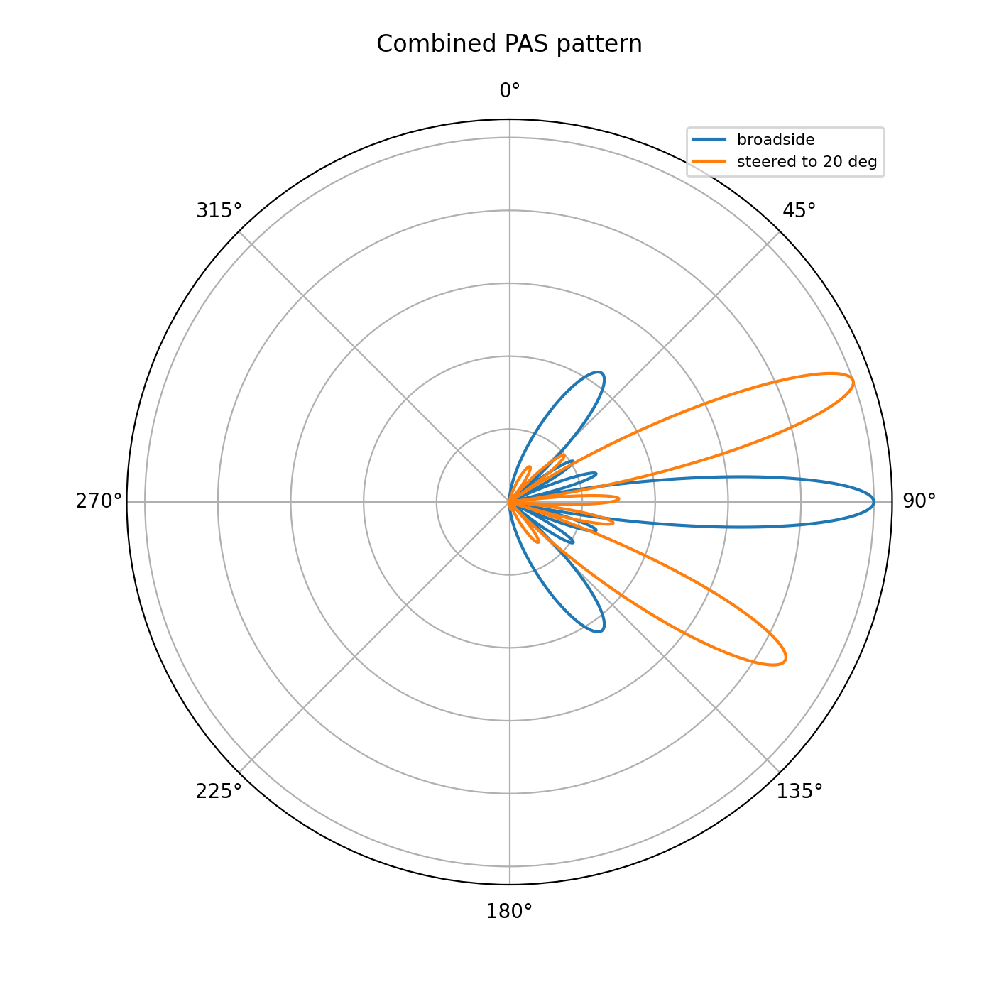
Use pas_pattern for design figures. Use array_factor alone when you want to isolate what the array geometry contributes independently of the finite dipole element pattern.

11.19.9. Directivity

sdas_directivity treats the element pattern as a radiation intensity, \(U(\theta) = F(\theta)^2\), and applies the standard antenna definition of directivity – peak intensity over the intensity averaged across all directions:

\[D_0 = \frac{4\pi\,U_{\max}}{P_\mathrm{rad}}, \qquad P_\mathrm{rad} = \int_0^{2\pi}\!\!\int_0^{\pi} U(\theta)\sin\theta \, d\theta \, d\phi = 2\pi \int_0^{\pi} U(\theta)\sin\theta\, d\theta,\]

evaluated numerically over n_theta samples in \(\theta\). A perfectly omnidirectional source has \(U(\theta)\) constant, which drives \(D_0 \to 1\); a larger value means more of the radiated power is concentrated near the peak direction rather than spread evenly in \(4\pi\) steradians.

>>> from pycsamt.emtools import sdas_directivity
>>> freq = 1024.0
>>> rho = 300.0
>>> k = wavenumber(freq, rho=rho)
>>> for length in (500.0, 1000.0, 2000.0, 5000.0):
...     directivity = sdas_directivity(length, k=k, n_theta=2000)
...     print(f"length={length:7.0f} m  directivity={directivity:.3f}")
...
length=    500 m  directivity=1.544
length=   1000 m  directivity=1.703
length=   2000 m  directivity=3.039
length=   5000 m  directivity=2.985

Do not assume that a longer dipole is always better. Directivity climbs from 1.544 to 3.039 between 500 m and 2000 m, but the 5000 m dipole comes back down to 2.985 – once length becomes a significant fraction of wavelength, directivity can change non-monotonically with frequency and length.

11.19.10. SNR Gain

snr_gain_db returns the coherent PAS gain relative to one SDAS:

\[G_\mathrm{dB} = 20 \log_{10}(N)\]

>>> from pycsamt.emtools import snr_gain_db
>>> for n_elem in (1, 2, 4, 8, 16):
...     print(f"N={n_elem:2d}: {snr_gain_db(n_elem):5.2f} dB")
...
N= 1:  0.00 dB
N= 2:  6.02 dB
N= 4: 12.04 dB
N= 8: 18.06 dB
N=16: 24.08 dB

This is the ideal coherent-array gain. It does not guarantee that all extra energy reaches the intended area. If grating lobes are present, a large fraction of the gain can be radiated into an unintended direction – as the previous section’s -30.92 degree lobe would do at 1024 Hz.

11.19.11. Plotting Patterns

plot_radiation_pattern accepts one pattern or a stack/list of patterns. It can draw polar plots for quick design review or Cartesian dB plots for side-lobe inspection.

>>> theta_b = np.linspace(-90.0, 90.0, 721)
>>> k = wavenumber(1024.0, rho=300.0)
>>> d = 2000.0
>>> patterns = [array_factor(theta_b, N=n, d=d, k=k) for n in (2, 4, 8)]
>>> fig, axes = plt.subplots(1, 2, figsize=(12, 4))
>>> _ = plot_radiation_pattern(
...     theta_b,
...     patterns,
...     labels=["N=2", "N=4", "N=8"],
...     polar=False,
...     ax=axes[0],
...     title="Linear amplitude",
... )
>>> _ = plot_radiation_pattern(
...     theta_b,
...     patterns,
...     labels=["N=2", "N=4", "N=8"],
...     polar=False,
...     log_scale=True,
...     db_floor=-40.0,
...     ax=axes[1],
...     title="dB view",
... )
>>> fig.tight_layout()
>>> fig.savefig("source_array_pattern_views.png", dpi=200)
>>> plt.close(fig)

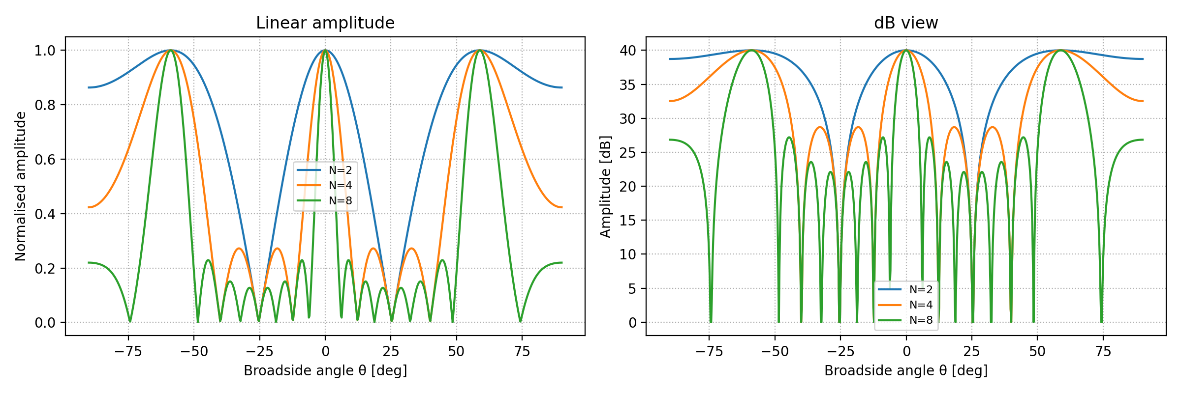
Use the dB view when side lobes matter. A weak-looking side lobe on a linear-amplitude plot may still be too strong for a field design.

11.19.12. Design Checklist

For a concrete PAS design, keep the calculation explicit:

>>> freq = 1024.0
>>> rho = 300.0
>>> N = 8
>>> d = 2000.0
>>> length = 1000.0
>>> target_angle = 25.0
>>> theta_b = np.linspace(-90.0, 90.0, 1801)
>>> k = wavenumber(freq, rho=rho)
>>> wavelength = 2.0 * np.pi / k
>>> beta = beam_steer(target_angle, d=d, k=k)
>>> lobes = steering_angles(N=N, d=d, k=k, beta=beta, n_range=4)
>>> pattern = pas_pattern(theta_b, N=N, d=d, k=k, beta=beta, l=length)
>>> print(f"earth wavelength = {wavelength:.1f} m")
earth wavelength = 1711.6 m
>>> print(f"d / wavelength = {d / wavelength:.3f}")
d / wavelength = 1.168
>>> print(f"beta = {beta:.4f} rad")
beta = -3.1028 rad
>>> print(f"steering-angle solutions = {lobes}")
steering-angle solutions = [-25.6707  25.    ]
>>> print(f"ideal coherent SNR gain = {snr_gain_db(N):.2f} dB")
ideal coherent SNR gain = 18.06 dB
>>> ax = plot_radiation_pattern(
...     theta_b,
...     pattern,
...     polar=False,
...     log_scale=True,
...     title="Final PAS design check",
... )
>>> ax.figure.savefig("final_pas_design_check.png", dpi=200)
>>> plt.close(ax.figure)

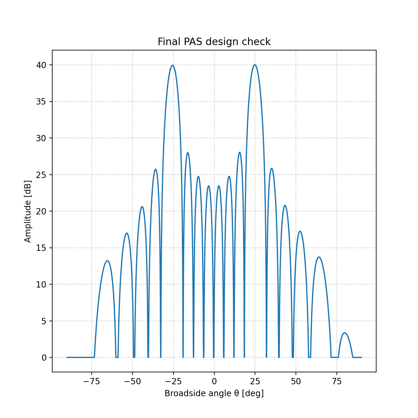
Review the output in this order:

• d / wavelength tells you whether grating lobes are physically plausible.

• steering_angles tells you where all main-lobe solutions are.

• The radiation pattern shows main-lobe width and side-lobe strength.

• snr_gain_db tells you the ideal coherent gain from element count.

Doubling N from 4 to 8 raised the grating lobe count from one (-30.92 degrees, above) to two (-25.67 and the intended 25.0 degrees is now paired with a mirror solution) – more elements buy more coherent gain, 18.06 dB here versus 12.04 dB at N=4, but at this same 1.168-wavelength spacing they do not buy a cleaner pattern.

11.19.13. Applying The Checklist To A Real CSAMT Survey

Every example above chose freq and rho freely. A real deployment does not have that freedom: the frequency band comes from the instrument program, and the representative resistivity comes from the ground itself. pyCSAMT’s bundled data/CSAMT line is real grounded dipole transmitter data from a groundwater-exploration survey in the Tongkeng area, Hunan Province, China (Kouadio et al., 2020) [Kouadio2020] – the same ten-station line used in CSAMT Field-Zone Classification. That page’s field-zone classification is the right tool for choosing a trustworthy resistivity here: at this survey’s roughly 1 km transmitter-receiver offset, most frequencies are near- or transition-field, where apparent resistivity is biased by source geometry rather than the earth alone. Restricting to the frequencies classified far keeps only physically meaningful resistivity for a wavenumber estimate.

>>> from pycsamt.emtools.fieldzone import classify_field_zones
>>> zones = classify_field_zones(
...     "data/CSAMT",
...     source_offset=1000.0,
...     far_threshold=3.0,
...     near_threshold=0.3,
...     recursive=False,
...     on_dup="replace",
...     strict=False,
...     verbose=0,
... )
>>> freqs_hz = np.sort(zones["freq_hz"].unique())
>>> print(freqs_hz.size, "frequencies,", freqs_hz.min(), "to", freqs_hz.max(), "Hz")
17 frequencies, 0.125 to 8196.722 Hz
>>> far = zones[zones["zone"] == "far"]
>>> sorted(far["freq_hz"].unique())
[2049.18, 4098.361, 8196.722]
>>> rho_rep = float(far["rho_a_ohmm"].median())
>>> print(f"representative far-field rho_a = {rho_rep:.1f} ohm.m")
representative far-field rho_a = 1170.0 ohm.m

Only the top three frequencies of this ten-station line ever classify as far field at a 1 km offset – everything below about 2 kHz would give an apparent resistivity contaminated by source geometry, not a number a transmitter-design wavenumber should be built on. The median resistivity across those trustworthy rows, 1170 \(\Omega\cdot\mathrm{m}\), is the representative half-space value carried into the rest of this section, in place of the arbitrary rho=300 used earlier on this page.

With a defensible resistivity in hand, check candidate element spacings across the survey’s entire real frequency band – not just two illustrative points – to see where in that band grating lobes would actually threaten a transmitter deployed on this line.

>>> d_candidates = (500.0, 1000.0, 2000.0)
>>> k_by_freq = np.array([wavenumber(f, rho=rho_rep) for f in freqs_hz])
>>> wavelength_by_freq = 2.0 * np.pi / k_by_freq
>>> for d in d_candidates:
...     ratio = d / wavelength_by_freq
...     n_grating = int(np.sum(ratio >= 1.0))
...     if n_grating:
...         fmin_grating = freqs_hz[ratio >= 1.0].min()
...         print(f"d={d:6.0f} m: d/wavelength = {ratio.min():.3f}-{ratio.max():.3f}, "
...               f"grating-lobe risk from {fmin_grating:.1f} Hz ({n_grating}/{freqs_hz.size})")
...     else:
...         print(f"d={d:6.0f} m: d/wavelength = {ratio.min():.3f}-{ratio.max():.3f}, "
...               "no grating-lobe risk in this band")
...
d=   500 m: d/wavelength = 0.002-0.419, no grating-lobe risk in this band
d=  1000 m: d/wavelength = 0.003-0.837, no grating-lobe risk in this band
d=  2000 m: d/wavelength = 0.007-1.674, grating-lobe risk from 4098.4 Hz (2/17)

>>> fig, ax = plt.subplots(figsize=(7.5, 4.2))
>>> for d in d_candidates:
...     _ = ax.plot(freqs_hz, d / wavelength_by_freq, "o-", label=f"d = {d:.0f} m")
...
>>> _ = ax.axhline(1.0, color="0.3", ls="--", lw=1.0)
>>> ax.set_xscale("log")
>>> _ = ax.set_xlabel("Frequency (Hz)")
>>> _ = ax.set_ylabel("d / wavelength")
>>> _ = ax.set_title("Grating-lobe risk across the real Tongkeng CSAMT band")
>>> _ = ax.legend()
>>> ax.grid(True, alpha=0.3, which="both")
>>> fig.tight_layout()
>>> fig.savefig("tongkeng_grating_lobe_risk.png", dpi=200)
>>> plt.close(fig)

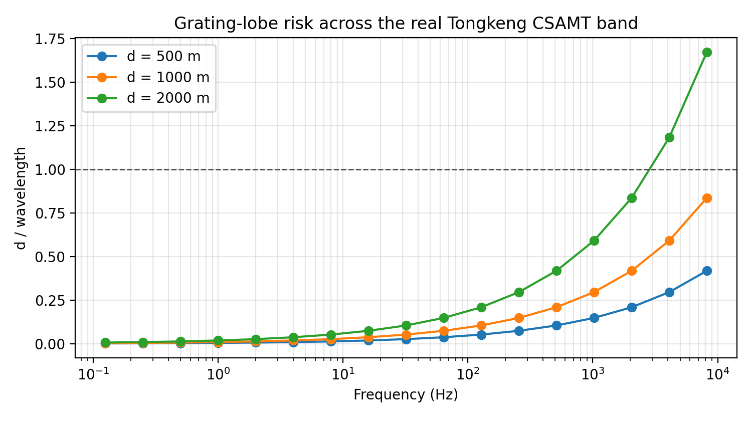
A 500 m or 1000 m element spacing stays comfortably under one wavelength across the entire real 0.125-8196.722 Hz program – the 1000 m curve only approaches the dashed grating-lobe line at the very top of the band, never crossing it. A 2000 m spacing, the value used for illustration throughout this page, crosses that line at the two highest real frequencies acquired on this line. For a transmitter array actually built for a survey like this one, that is the concrete, data-grounded reason to prefer the shorter spacing, or to accept that the top two frequencies need separate grating-lobe review – not an assumption made in the abstract.

11.19.14. Common Pitfalls

Do not design from free-space wavelength at CSAMT frequencies. Use wavenumber(freq, rho=...) when a representative resistivity is available.

Do not check only one frequency. A layout with modest spacing at low frequency can have d / wavelength > 1 at the high end of the sweep.

Do not treat SNR gain as directional selectivity. snr_gain_db(8) is about 18 dB, but grating lobes can send much of that coherent energy away from the intended target.

Do not mix the angle conventions. sdas_element_pattern uses angle from the dipole axis; array_factor and pas_pattern use broadside angle.

Do not carry an apparent resistivity straight from field data into a wavenumber estimate without checking its field zone first – a near-field-biased value can distort the whole design, as the Tongkeng example above demonstrates.

11.19.15. Worked Example

The example walks through the single-dipole pattern, earth versus free-space wavenumber, low- and high-frequency array factors, beam steering, grating-lobe detection, combined PAS patterns, directivity, SNR gain, and one concrete 8-element design.

Open the rendered gallery page here: Phased-array CSAMT transmitter design (pycsamt.emtools.source_array).