
4.1. Loading Map Data#
The mapping package uses one normalized object,
pycsamt.map.MapData, for every station map, profile
pseudosection, and 3-D view. In the documentation this object
is also referenced as MapData: the loader’s reproducible record
of stations, profile membership, source objects, and metadata. You
rarely need to build it by hand. Most public plotting functions accept
the same inputs directly and call the normalizer for you.
Use this page when you want explicit control over loading, line grouping, or pre-flight checks before drawing a map.
4.1.1. Loading Philosophy#
The loader follows the science API rather than the web app internals.
It delegates EDI parsing to
pycsamt.emtools._core.ensure_sites(), then extracts the small
mapping contract needed by the renderers:
station identifier;
latitude, longitude, and elevation when available;
profile or survey-line name;
the original EDI-like object, including its impedance tensor
Zobject.
This means a code workflow and the web workflow can start from the same survey files, but code users can inspect, group, transform, and export each intermediate object. The contract is deliberately small: if station \(i\) is normalized as \(s_i=(\mathrm{id}_i,\phi_i,\lambda_i,h_i,\ell_i,i)\), then the renderers read the same station identifier, latitude \(\phi_i\), longitude \(\lambda_i\), elevation \(h_i\), line name \(\ell_i\), and zero-based index \(i\) everywhere. That shared tuple is what keeps station, profile, and 3-D views from silently disagreeing about order or line membership.
4.1.2. Input Types#
All loading helpers accept flexible EDI sources:
strorpathlib.PathA single EDI file or a directory containing EDI files.
- sequence of paths
A list or tuple of EDI files. A sequence of directories is treated as one line per directory by
pycsamt.map.load_lines().- EDI-like iterable
EDI-like object instances with station metadata and a
Zattribute, including objects already loaded elsewhere in pyCSAMT.Sites-like containerAny object accepted by
ensure_sites. Containers exposingas_list()are unpacked into EDI-like objects.MapDataReturned unchanged, so it is safe to pass normalized data through higher-level builders.
Regardless of the input form, the normalizer tries to produce the same mathematical object: an ordered station set \(S=(s_0,\ldots,s_{N-1})\) and a partition of that set into profile lines \(L_1,\ldots,L_K\). A partition means each station belongs to one resolved line, while the combined survey still keeps the global index \(i\) needed for reproducible sorting and exports.
4.1.3. Single-Line Loading#
For one profile line, call pycsamt.map.ensure_map_data()
directly or pass the source to a plotting helper.
>>> from pycsamt.map import (
...     StationMapOptions,
...     ensure_map_data,
...     plot_station_map,
... )

>>> source = "data/AMT/WILLY_DATA/L18PLT"

>>> data = ensure_map_data(source, recursive=True)
>>> print(data.station_ids)
('18-001A', '18-002U', '18-003A', '18-004A', '18-005U', '18-006A', '18-007U', '18-008U', '18-009A', '18-010U', '18-011A', '18-012A', '18-013U', '18-014A', '18-015U', '18-016A', '18-017U', '18-018A', '18-019U', '18-020A', '18-021U', '18-021B', '18-022U', '18-022V', '18-023A', '18-023V', '18-024U', '18-025A')
>>> print(data.lines)
('line',)
>>> print(data.has_geo)
True

>>> options = StationMapOptions(
...     backend="matplotlib",
...     overlay="elevation",
...     title="L18 station map",
... )
>>> fig = plot_station_map(data, options=options)
The three printed values confirm that station order, line membership, and geographic coverage survived normalization. The same normalized records produce the static map below; explicitly setting the overlay is important because the default color variable is station index, not elevation.
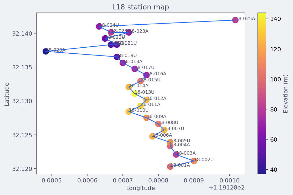
Station locations loaded from data/AMT/WILLY_DATA/L18PLT and
colored by elevation. The line doubles back near its northern end,
and several labels overlap there; both features come from the survey
geometry rather than from loading errors. The elevation colors vary
independently of that geometry, with the highest part of the line
concentrated around stations 18-011A to 18-014A.#
ensure_map_data does not force every station to have geographic
coordinates. data.has_geo tells you whether all normalized
stations have finite latitude and longitude. If coordinates are
missing, profile views can still use station order or distance, while
geographic station maps may need CRS or coordinate preprocessing. In
set notation, data.has_geo is true only when
\(\phi_i,\lambda_i \in \mathbb{R}\) for every station
\(s_i \in S\); missing or non-finite coordinates are represented as
None before a renderer decides how to proceed.
4.1.4. Multiple-Line Loading#
Use pycsamt.map.load_lines() when a survey is split across
several folders or when you want one combined object for 3-D fence,
block, or depth-slice views.
>>> from pycsamt.map import load_lines

>>> data = load_lines(
...     "data/AMT/WILLY_DATA",
...     detect="folder",
...     recursive=True,
... )

>>> print(data.lines)
('L18PLT', 'L22PLT', 'L26PLT', 'L30PLT', 'L34PLT')
>>> print(data.metadata["n_lines"])
5
>>> print(data.station_ids[:5])
('18-001A', '18-002U', '18-003A', '18-004A', '18-005U')
Each station is re-indexed across the combined survey and tagged with
its resolved line name. The renderers then use data.profiles to
draw separate profiles or offset lines in 3-D. For five loaded lines,
the combined station set is still one sequence
\(S=(s_0,\ldots,s_{N-1})\), but each station carries a line label
\(\ell_i \in \{L18PLT,L22PLT,L26PLT,L30PLT,L34PLT\}\). This is
why a station map can show all stations together while a fence or
pseudosection view can split them back into their profile lines.
4.1.5. Grouping Modes#
When load_lines receives one directory, the detect option
decides how files become lines.
detect="folder"Group by immediate parent folder. This is the best option for layouts such as
WILLY_DATA/L18PLT/*.ediandWILLY_DATA/L22PLT/*.edi. A flat folder becomes one line named after the folder.detect="flat"Treat every discovered EDI file under the directory as one line. Use this for a single profile stored in a nested directory tree.
detect="auto"Group by station-ID prefix. Numeric prefixes are normalized with an
Lprefix. For example, station files beginning with22are grouped underL22. Use this when line folders are not reliable but station naming is consistent.
You can inspect the grouping without loading impedance data by calling
pycsamt.map.resolve_line_groups().
>>> from pycsamt.map import resolve_line_groups

>>> groups = resolve_line_groups(
...     "data/AMT/WILLY_DATA",
...     detect="folder",
... )

>>> for line, source in groups.items():
...     print(line, len(source))
L18PLT 28
L22PLT 25
L26PLT 25
L30PLT 25
L34PLT 25
The grouping operation is simply the line partition before data
normalization. For a directory source \(D\), detect="folder"
maps each discovered EDI path \(p\) to the immediate parent name
\(g(p)\). detect="flat" uses one constant group for all paths,
and detect="auto" derives \(g(p)\) from the station-name prefix.
Writing that rule down matters for reproducibility because changing
only the grouping rule can change profile labels even when the EDI
files are identical.
4.1.6. Explicit Line Mapping#
The most reproducible multi-line workflow is an explicit mapping:
>>> from pycsamt.map import load_lines

>>> data = load_lines({
...     "L18": "data/AMT/WILLY_DATA/L18PLT",
...     "L22": "data/AMT/WILLY_DATA/L22PLT",
...     "L26": "data/AMT/WILLY_DATA/L26PLT",
... })
>>> print(data.lines)
('L18', 'L22', 'L26')
>>> print(len(data.stations))
78
Mapping values may be directories, file lists, or EDI-like iterables. This is useful in notebooks and scripts where line names should be stable even if folder names later change. An explicit mapping fixes the function \(g(p)=\ell\) in the script itself, so the line label comes from the mapping key rather than from a mutable folder name.
If your EDI-like objects do not carry line metadata, but you already
know station membership, pass line_map to
pycsamt.map.ensure_map_data().
>>> from pycsamt.map import ensure_map_data

>>> data = ensure_map_data(
...     edis,
...     line_map={
...         "L18": ["S001", "S002", "S003"],
...         "L22": ["S101", "S102", "S103"],
...     },
... )
Line metadata embedded on the EDI object takes priority. The fallback order is:
line;profile;survey_line;Line;Profile;station lookup in
line_map;default line name
"line".
That priority order is deterministic. If two sources could assign a line name, the first non-empty value in the list wins, and the resulting line label is stored on each station record.
4.1.7. Normalized Contract#
MapData exposes the surface that all map renderers share. A compact inspection avoids printing the full EDI objects:
>>> print(type(data.station_ids).__name__, len(data.station_ids))
tuple 78
>>> print(data.lines, data.has_geo)
('L18', 'L22', 'L26') True
>>> print(len(data.iter_edis()), len(data.stations), len(data.profiles))
78 78 3
Each pycsamt.map.StationRecord contains one
station record:
>>> station = data.stations[0]
>>> print(
...     station.id, station.latitude, station.longitude,
...     station.elevation, station.line, station.index,
... )
18-001A 32.1203 119.12883333333333 99.0 L18 0
station.source is the original EDI-like object. Keep it when you
need to inspect impedance arrays, frequencies, or file-level metadata
after loading.
The profile contract is similarly compact. Each
pycsamt.map.ProfileLine is a profile line with a
name and an ordered tuple of stations. The order is the loader
order, so any derived coordinate such as along-line station number is
reproducible from the normalized object.
4.1.8. Pre-Flight Checks#
A good loading workflow checks the normalized survey before plotting:
>>> from pycsamt.map import (
...     ensure_map_data,
...     select_frequency,
...     value_at_frequency_details,
... )

>>> data = ensure_map_data("data/AMT/WILLY_DATA/L18PLT")
>>> first_edi = data.iter_edis()[0]
>>> freq = first_edi.Z.freq
>>> selection = select_frequency(freq, requested=100.0)

>>> if selection is None:
...     raise RuntimeError("No finite positive frequency was found.")

>>> print("requested:", selection.requested)
requested: 100.0
>>> print("actual:", selection.actual)
actual: 102.4
>>> print("relative delta:", selection.relative_delta)
relative delta: 0.024000000000000056

>>> values = value_at_frequency_details(
...     data,
...     frequency=selection.actual,
...     quantity="rho",
...     component="xy",
... )
>>> print("stations with values:", len(values))
stations with values: 28
This is especially helpful when different stations have slightly different frequency grids. Map extraction chooses the nearest finite positive frequency per station and can enforce a tolerance when you need a strict match. For a requested frequency \(f_r\) and a station grid \(F_i=\{f_{i0},\ldots,f_{im}\}\), the selected sample is
Equation (1) makes the selection deterministic; if two samples are equally near, NumPy’s first-minimum rule selects the first one in the recorded array. The reported relative delta is \(|f_i^\*-f_r|/|f_r|\) when \(f_r\) is positive. Once the frequency index is selected, the requested impedance tensor component is read from
where component="xy" selects \(Z_{xy}\) in
(2). EDI parsing has already converted
that component into apparent resistivity and phase arrays. Their field-unit
convention is
The map extractor reads the stored \(\rho_{a,ab}\) or \(\varphi_{ab}\) at index \(k_i\); it does not recompute them. Consequently, another user needs the same input EDI files, requested \(f_r\), component, quantity, and tolerance to reproduce the values.
4.1.9. Handling Missing or Partial Data#
The loader is designed for field surveys, where not every file is perfect.
Files without valid impedance are skipped by value-extraction helpers instead of breaking the whole map.
Non-finite coordinates become
NoneonStationRecord.If no line name is available, stations are grouped into
"line".Empty groups are ignored by
load_lines.A
MapDatawith no stations is still a valid object; renderers can return empty figures rather than crashing.
For strict workflows, validate the counts yourself:
>>> data = load_lines("data/AMT/WILLY_DATA", detect="folder")

>>> if not data.stations:
...     raise RuntimeError("No stations were loaded.")
>>> if not data.has_geo:
...     raise RuntimeError("Station map requires geographic coordinates.")
>>> if len(data.lines) < 2:
...     raise RuntimeError("Expected a multi-line survey.")
>>> print(f"ready: {len(data.stations)} stations on {len(data.lines)} lines")
ready: 128 stations on 5 lines
4.1.10. Using Loaded Data#
Once loaded, pass the same MapData object to station, profile, and
3-D builders. This avoids re-reading files and keeps grouping
consistent across views. The station-map example earlier on this page
shows that hand-off and its rendered result; Station Maps,
Profile Maps And Pseudosections, and 3-D Quick-Look Maps develop the corresponding views
without repeating their figures here.
Use the export helpers to save any resulting figure:
>>> from pycsamt.map import write_html

>>> write_html(station_fig, "outputs/stations.html")
write_html returns None, so a successful call has no terminal
output. Its observable result is outputs/stations.html.
4.1.11. Troubleshooting#
FileNotFoundErrorThe path passed to
load_linesorensure_map_datadoes not exist. Resolve project-relative paths before loading.ValueError: Unknown detect modedetectmust be one of"folder","flat", or"auto".- No stations in the output
Check that EDI files were discovered and that
ensure_sitescan read them. Start withresolve_line_groupsto confirm grouping.- Station map is empty
Inspect
data.has_geo. Geographic maps require finite latitude and longitude unless you first reproject or provide coordinates.- Pseudosection has gaps
Some stations may be missing impedance values, or the requested frequency/period may not be present within tolerance. Inspect
value_at_frequency_detailsfor selected-frequency metadata.