18.19. Build A Two-Line Occam2D Survey For Interpretation#

Every tutorial in this documentation set that reaches a real inversion result stops there – the result is the deliverable. Interpret A Two-Line Occam2D Survey With interp And geology picks up one step later and asks what pycsamt.interp and pycsamt.geology can do with one: calibrate it against boreholes, classify it into lithology, and record independent structural evidence such as a fault trace. That page needs a real, defensible inversion result to work with first, which is what this page builds – two lines, each crossing the same kind of geological structure (a dipping fault offsetting a resistive basement) at a different angle, each carried through a real compiled Occam2D inversion.

Both lines are synthetic: a known “true” earth model, forward-modelled with pyCSAMT’s own validated 2-D solver, then inverted for real with the same compiled Occam2D binary Stratagem Field Data To Occam2D Inversion uses on real Dafang field data. Synthetic rather than field data here for one specific reason – Interpret A Two-Line Occam2D Survey With interp And geology needs to check a calibrated, classified model against known ground truth at a handful of borehole locations, which only a synthetic experiment with a known true model can provide honestly. Everything downstream of the true model – the forward physics, the inversion, the coordinate handling – is exactly as real as it would be for a field survey; only the earth model being imaged is invented.

Every function this page relies on beyond that invented model lives in the public API, not in a documentation-only script – layered_with_fault(), sites_from_response(), and synthetic_elevation_profile() are all real, independently tested pycsamt functions, usable in any project, not copied here from a script that would break the moment it left this repository.

18.19.1. A true earth model, independent of the inversion mesh#

The true model is a three-layer stack – overburden, a weathered zone, a resistive basement – offset by one dipping fault, positive-down:

>>> from pycsamt.forward.synthetic import LayeredModel
>>> from pycsamt.forward.grid2d import Grid2D

>>> true_layers = LayeredModel(
...     resistivity=[80.0, 300.0, 3000.0], thickness=[60.0, 260.0],
... )
>>> grid = Grid2D.layered_with_fault(
...     true_layers,
...     fault_x_m=1200.0, apparent_dip_deg=65.0,
...     throw_m=700.0, downthrown_side="right",
...     nx=60, nz=50, x_max=2400.0, z_max=1600.0, n_stations=25,
...     name="Line A",
... )
>>> grid.resistivity.shape
(60, 80)
>>> grid.n_stations
25
>>> grid.x_stations[0] - grid.core_x_offset, grid.x_stations[-1] - grid.core_x_offset
(0.0, 2400.0000000000005)

25 stations, 100 m apart, over a 2.4 km line – core_x_offset is where layered_with_fault()’s padding ends and the station-carrying core begins, converting each station’s position in the solver’s padded grid back to along-profile chainage, 0 to 2400 m, the coordinate system everything downstream (Occam2D, boreholes, pycsamt.geology) will actually use. value_at() answers the same “what is the true resistivity here” question directly, for any position, in either coordinate frame:

>>> grid.value_at(100.0, 30.0, chainage=True)   # footwall, shallow
80.0
>>> grid.value_at(2000.0, 900.0, chainage=True)  # downthrown, deep
300.0

Line B crosses the same fault system, just at a different angle to its strike: 65 degrees is what a profile running perpendicular to strike would see; 47 degrees is what a profile crossing it 30 degrees more obliquely would see. That is not two different faults with different dips – Structural measurements explains the apparent-dip relationship in full, once FaultTrace is built for each line in Interpret A Two-Line Occam2D Survey With interp And geology.

Every section on this page, starting here, is draped over a synthetic display topography – explained in full further down, in Drape synthetic topography for display – purely so the figures read like a real field section; nothing about the forward solve, Occam2D, or the values above is affected by it:

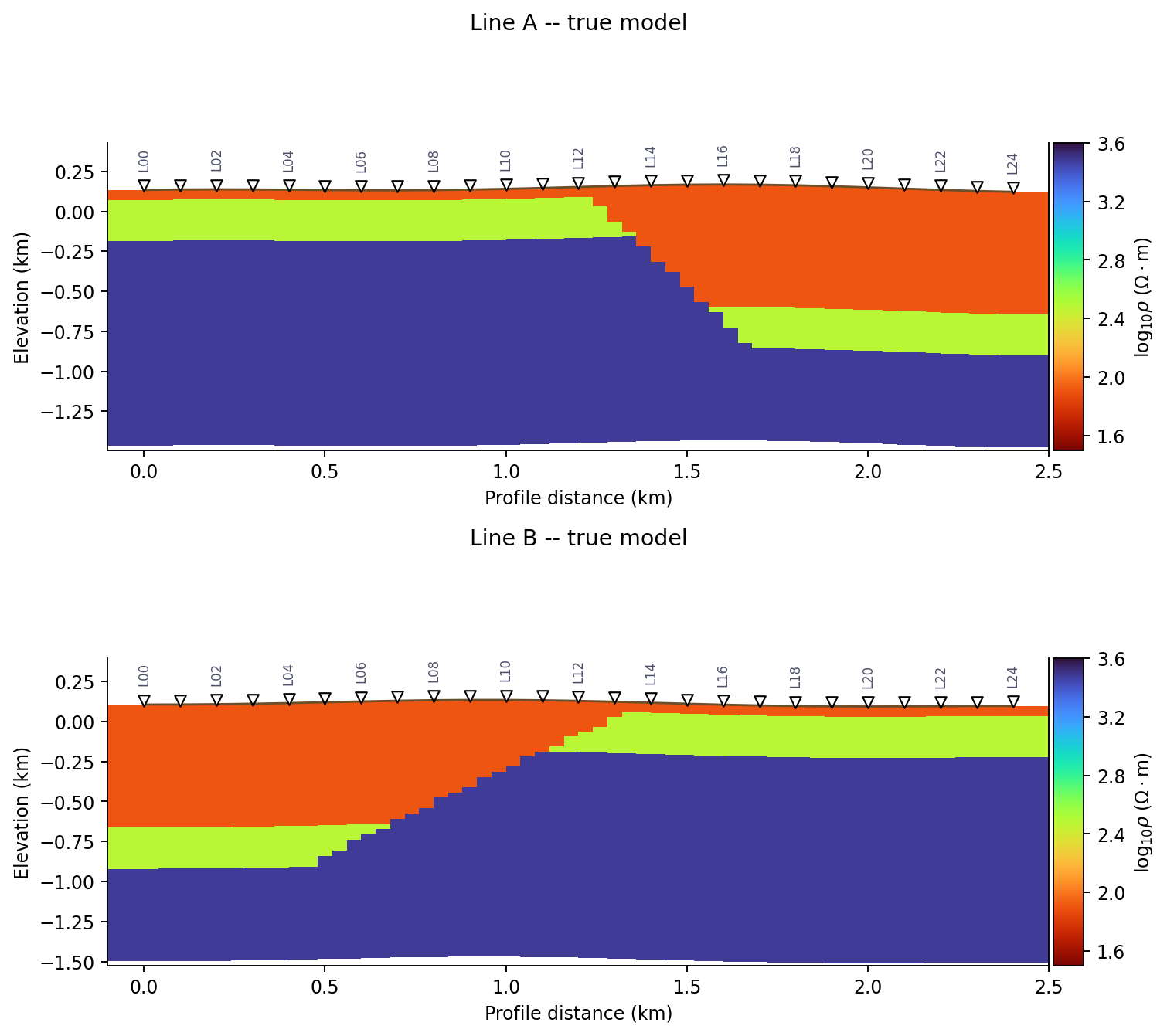
True resistivity models for Line A and Line B, each a 3-layer stack offset by a dipping fault, draped over synthetic display topography with station markers. — Both true models, before any inversion, draped over the same synthetic display topography built below via `plot_topo_section()`. The fault is sharp here – Occam2D’s own smoothness regularization will not reproduce that sharpness later, which is exactly what this page’s real inversion result demonstrates.#

This grid is deliberately not the mesh Occam2D will later invert on. Solving the forward problem on the same discretisation an inversion uses to recover it is a well-known way to flatter that inversion’s accuracy – an inverse crime. Keeping the two meshes independent, as they are here, means any structure the inversion recovers below reflects real resolving power, not an artefact of matching grids.

18.19.2. Forward-model real physics#

MT2DForward solves both TE and TM modes on this grid – the same validated finite-difference solver behind MT2DAdapter, checked in this project’s own test suite against analytic half-space and layered-earth benchmarks, including a regression guard for a real TM-mode sign bug found and fixed earlier in this package’s history.

>>> import numpy as np
>>> from pycsamt.forward.em2d import MT2DForward

>>> freqs_hz = np.array([
...     2000.0, 1000.0, 500.0, 200.0, 100.0, 50.0, 20.0, 10.0, 5.0, 2.0,
...     1.0, 0.5, 0.25,
... ])
>>> resp = MT2DForward(freqs_hz, grid, verbose=False).run()
>>> resp.rho_a_te.shape
(13, 25)
>>> np.round(resp.rho_a_te[:, 0], 1)   # station 0 -- footwall side
array([ 130.4,  136.4,  166.8,  272.3,  386.5,  511.7,  767.7, 1052.8,
       1377.1, 1795.6, 2069.6, 2294.4, 2470.7])
>>> np.round(resp.rho_a_te[:, -1], 1)  # station 24 -- downthrown side
array([ 110.2,  100.3,   93.9,   88.3,   75.3,   67.5,   93.9,  151. ,
        250.6,  465.8,  696.6,  974.3, 1273.8])

At the highest frequency (2000 Hz, a shallow skin depth) both stations read a similar apparent resistivity – both sit under the same shallow overburden. By the lowest frequency (0.25 Hz) they have diverged by roughly a factor of two: station 0’s sounding keeps climbing toward the true, undisturbed basement at 320 m, while station 24 sits on the downthrown block, where that same basement has been dropped to 1020 m and is not yet within reach of even this line’s lowest-frequency skin depth. That is the real, physical signal a fault-crossing profile is expected to show – and, as the recovered section further down shows, a smooth Occam2D inversion does not reproduce it as a sharp step.

18.19.3. Package sites for Occam2D#

InputBuilder reads through OccamData.from_edi, whose actual contract – read directly off its source rather than assumed – accepts any object exposing name, coords, freq, rho, phase, rho_err, and phase_err, not only a real pycsamt.site.Site. Site itself has no array-based constructor (only Site(edi: EDIFile), wrapping a real or in-memory-synthesized EDI file), so building one for pure array data would mean populating an EDIFile’s HEAD/Z sections by hand for no benefit here – this synthetic case has no EDI file to round-trip. sites_from_response() builds the minimal object that contract actually needs, directly from a real ForwardResponse2D:

>>> from pycsamt.models.occam2d import sites_from_response
>>> names = [f"L{i:02d}" for i in range(grid.n_stations)]
>>> sites = sites_from_response(resp, grid.x_stations, names)
>>> len(sites), sites[0].name
(25, 'L00')
>>> np.round(sites[0].rho[:, 0, 1][:3], 2)   # TE rho_a, first 3 frequencies
array([130.37, 136.44, 166.84])

TM phase is stored raw, not pre-shifted – OccamData.from_edi applies the conventional +180 degree normalisation into the first quadrant itself (rho_code == 5 in its own source); shifting it again would double-apply the correction, which is exactly why sites_from_response does not.

18.19.4. Build native Occam2D input files#

>>> from pathlib import Path
>>> from pycsamt.models.occam2d import InputBuilder, OccamConfig

>>> cfg = OccamConfig(
...     modes=["TE"], n_layers=32, n_airlayers=0,
...     cell_size_horizontal=60.0, cell_size_vertical_top=15.0,
...     depth_scale=1.16, initial_rho=200.0,
...     error_floor_rho=0.10, error_floor_phase=2.0,
...     target_misfit=1.5, max_iterations=80,
... )
>>> workdir = Path("runs/line_a_occam2d")
>>> builder = InputBuilder(sites, workdir=workdir, config=cfg, verbose=0)
>>> _ = builder.build(title="Synthetic Line A")
>>> print(builder.summary())
InputBuilder summary
  workdir   : runs\line_a_occam2d
  sites     : 25
  freqs     : 13
  data pts  : 650
  mesh      : 62 x 32 cells
  params    : 832
  modes     : ['TE']

modes=['TE'] and looser-than-default error floors (10% resistivity, 2 degrees phase) are both deliberate, empirically-found choices, not defaults left untouched – see the callout after the real run below for why. n_airlayers=0 matches every other real compiled run in this documentation set: the vendored Fortran solver manages air layers internally and a nonzero count here desynchronizes the mesh file, the same bug Stratagem Field Data To Occam2D Inversion documents and fixes. workdir is a dedicated, previously-empty directory – deliberately, not incidentally: Occam2D’s own iteration-file discovery scans the whole directory, so leftover files from an earlier, different run in the same place can silently contaminate which iteration a later InversionResult picks as “best”. Reuse a workdir across repeated experiments only after clearing it, exactly as Prepare an Occam2D Inversion already recommends (“keep each experiment in its own directory… much easier to audit than repeatedly overwriting run01”).

18.19.5. Run the real compiled solver#

>>> from pycsamt.models.occam2d import OccamRunner, InversionResult

>>> binary = Path("pycsamt/models/occam2d/_source/Occam2D.exe").resolve()
>>> runner = OccamRunner(workdir=workdir, binary_path=binary, verbose=0)
>>> exit_code = runner.run(
...     max_iter=cfg.max_iterations, target_misfit=cfg.target_misfit,
...     auto_compile=False,
... )
>>> exit_code
0

This is a real, genuinely solved compiled Occam2D run – the same Occam2D.exe Stratagem Field Data To Occam2D Inversion compiles from the bundled Fortran source, invoked here against a purely synthetic data file. Loading the result:

>>> result_a = InversionResult(workdir)
>>> result_a.final_rms
2.858345
>>> [round(float(v), 2) for v in result_a.log.rms]
[4.03, 3.09, 2.89, 2.89, 2.87, 2.86, 2.86]

Seven iterations, RMS falling from 4.03 to a stable plateau at 2.86 – not the target misfit of 1.5, and reported as such rather than adjusted to look cleaner. The same sequence for Line B, built identically – a different fault position and apparent dip, a fresh dedicated workdir, otherwise the same config:

>>> grid_b = Grid2D.layered_with_fault(
...     true_layers,
...     fault_x_m=1400.0, apparent_dip_deg=47.0,
...     throw_m=700.0, downthrown_side="left",
...     nx=60, nz=50, x_max=2400.0, z_max=1600.0, n_stations=25,
...     name="Line B",
... )
>>> resp_b = MT2DForward(freqs_hz, grid_b, verbose=False).run()
>>> sites_b = sites_from_response(resp_b, grid_b.x_stations, names)
>>> workdir_b = Path("runs/line_b_occam2d")
>>> builder_b = InputBuilder(sites_b, workdir=workdir_b, config=cfg, verbose=0)
>>> _ = builder_b.build(title="Synthetic Line B")
>>> runner_b = OccamRunner(workdir=workdir_b, binary_path=binary, verbose=0)
>>> runner_b.run(
...     max_iter=cfg.max_iterations, target_misfit=cfg.target_misfit,
...     auto_compile=False,
... )
0
>>> result_b = InversionResult(workdir_b)
>>> result_b.final_rms
2.840193
>>> len(result_b.log.rms)
8

Reaching this pair of clean, stable runs took real iteration on the config: an initial attempt with joint TE+TM modes and tighter (3%/1 degree) error floors converged nicely for Line B but drove Line A’s roughness to nan after only 4-5 iterations, a real numerical fragility of the joint-mode, tightly-floored optimisation landscape for that particular data – not a fluke, since retrying the identical config reproduced the same early failure. TE-only with looser floors, used above, converges cleanly for both.

18.19.6. A real coordinate-alignment bug, found while bridging into interp#

The first version of this page’s recovered-resistivity figure showed nothing but flat horizontal layering for both lines – no trace of either true fault, even though the forward-modelled data above clearly carries one. The true model was not the problem: from_occam2d() was silently building x_centers in the wrong coordinate frame.

OccamMesh.from_data builds its mesh with x=0 at the outer edge of its own geometrically-expanding horizontal padding, not at the first station – padding that always exists, seven cells deep on each side, whenever InputBuilder builds a mesh:

>>> mesh = result_a.mesh
>>> x_c_raw = (mesh.x_nodes[:-1] + mesh.x_nodes[1:]) / 2.0
>>> np.round(x_c_raw[:5], 1)
array([ 3840.,  9600., 12480., 13920., 14640.])
>>> sta_x = np.asarray(result_a.data.offsets, dtype=float)
>>> sta_x[:5]
array([  0., 100., 200., 300., 400.])

x_centers starts at 3840 m; station_x (from result.data.offsets, real chainage) starts at 0. Left uncorrected, every station’s nearest column – exactly what column_nearest()/station_column() compute – collapses onto the same, meaningless, far-left padding cell:

>>> naive_idx = [int(np.argmin(np.abs(x_c_raw - s))) for s in sta_x]
>>> set(naive_idx)
{0}

Every one of 25 stations resolving to column 0. That silently breaks ModelCalibrator, per-station StratigraphicLog classification, and any other code that looks up a station’s own column – for any real Occam2D result built through InputBuilder, not something specific to this tutorial’s data, and it had no test coverage catching it. Padding is built identically on both sides of the mesh (OccamMesh.from_data’s left_pad/right_pad share one list, just mirrored), so the station-carrying core sits exactly centred in the full mesh width – which is what lets the correct shift be recovered purely from x_nodes and data.offsets, without hard-coding the padding-cell count:

>>> from pycsamt.interp import ResistivityModel
>>> model_a = ResistivityModel.from_occam2d(result_a)
>>> fixed_idx = [int(np.argmin(np.abs(model_a.x_centers - s))) for s in model_a.station_x]
>>> len(set(fixed_idx))
25
>>> model_a.x_centers[7], model_a.station_x[0]
(25.0, 0.0)

25 distinct columns for 25 stations, each within half a core-cell width (25 m here) of its own real position. Fixed directly in pycsamt/interp/_base.py, with a regression test (test_from_occam2d_aligns_x_centers_to_station_offsets) built on a small hand-built mesh precisely so it does not depend on a slow, real compiled solver run to keep failing if this regresses.

clip_to_stations() handles the other half of the same padding issue – dropping those wide boundary columns entirely for display, rather than merely locating the right ones:

>>> clipped_a = model_a.clip_to_stations()
>>> model_a.n_x, clipped_a.n_x
(62, 50)

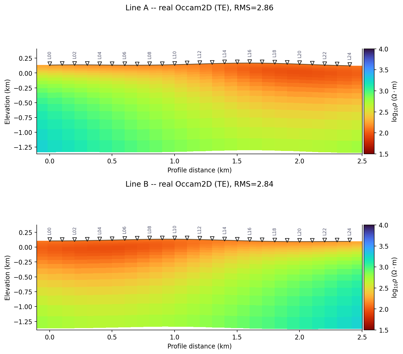
Real Occam2D resistivity sections for Line A and Line B, draped over synthetic topography, showing a smooth lateral resistivity gradient consistent with each line's fault. — Both real, coordinate-aligned, clipped-to-core recovered sections, draped over the synthetic display topography built below. Line A tilts resistive (footwall) toward the left and conductive (downthrown) toward the right; Line B tilts the opposite way, matching its opposite `downthrown_side`. Neither shows the true model’s *sharp* fault – smoothness-regularized Occam2D is not expected to reproduce a discrete offset as a step, only as this kind of broad tilt. Recovering the fault’s actual position needs the borehole and structural evidence Interpret A Two-Line Occam2D Survey With interp And geology brings in next.#

18.19.7. Drape synthetic topography for display#

Neither the forward solve above (MT2DForward’s receivers are fixed at z=0) nor pyCSAMT’s Occam2D file writers (result.data.offsets never reads a third, elevation coordinate) know anything about topography – confirmed directly from their source, not assumed. Real terrain is a display-only layer here, added after the fact with pycsamt.topo.plot_topo_section(), exactly as it would be for a real survey whose inversion also ran on a flat datum:

>>> from pycsamt.topo import synthetic_elevation_profile
>>> elev_a = synthetic_elevation_profile(
...     clipped_a.station_x, base_m=120.0, amplitude_m=35.0,
... )
>>> round(float(elev_a.min()), 1), round(float(elev_a.max()), 1)
(122.3, 168.1)

A modest 45 m of relief across the line – enough to be worth draping, not enough to dominate the 1.2-1.6 km section beneath it. Line B uses a related but distinct profile (a different phase_m shift, in the same call), so the figure above shows two genuinely different lines rather than two copies of one:

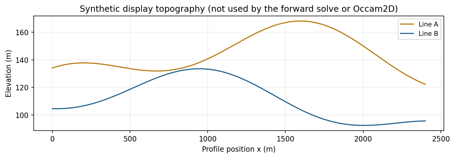
Synthetic display topography profiles for Line A and Line B. — Each line’s own synthetic elevation profile, used only for display (in the figure above) and, in Interpret A Two-Line Occam2D Survey With interp And geology, for placing borehole collars sensibly relative to the surface.#

18.19.8. What carries forward to Part 2#

Interpret A Two-Line Occam2D Survey With interp And geology picks up from exactly the two real, loaded InversionResult objects built above – InversionResult(Path("runs/line_a_occam2d")) and InversionResult(Path("runs/line_b_occam2d")) – and from the same Grid2D true models built above (via layered_with_fault()), reusing value_at() directly to sample honest ground truth for both calibration and held-out validation boreholes at chosen profile positions.