18.17. Forward Model One Real Line In 1-D, 2-D, And 3-D#

The Tongkeng CSAMT line – the same ten-station, 50 m-spaced, real field survey Map Groundwater Geology From CSAMT uses – is small enough to carry through every dimensionality pyCSAMT’s forward layer offers without substituting a single synthetic value. This tutorial does exactly that:

load the line and re-establish the trustworthy far/transition frequency band Map Groundwater Geology From CSAMT already derives for this survey, rather than re-deriving it;
build a real, Bostick-informed 1-D layered guess and forward model it with the legacy MT1DForward, against the real corrected sounding at one station;
benchmark the in-house triangular solver against that same layered model before trusting it on real geometry – and use what that benchmark finds to choose which frequencies the rest of this tutorial can honestly use;
drape that same layered guess over the line’s real station elevations with a real graded TriMesh, solve it, and compare the modelled response with the real corrected data at all ten stations;
embed the same real profile in a 3-D volume and solve it with a real compiled ModEM binary, closing the loop back to the 1-D analytic answer.

Unlike Map Groundwater Geology From CSAMT, nothing here trains a model or maps geology – the question this tutorial answers is narrower and more mechanical: what does each extra dimension actually buy, on this one real line, checked against this one real line’s own data at every step. See that tutorial for the AI-inversion and groundwater-mapping application built on the same survey.

18.17.1. What You Will Learn#

After this tutorial you should be able to:

reuse an already-established real near-field correction and trustworthy frequency band rather than re-deriving survey-specific corrections inside a forward-modelling exercise;
turn a real corrected sounding into a depth-resistivity curve with bostick_depth_from_rho(), and know why the sites-based bostick_depth() is the wrong tool for a single-component (Ex-Hy only) CSAMT survey specifically;
benchmark TriFEM2DAdapter against an exact analytic answer before trusting it on real data, and use a failed benchmark to choose a defensible frequency subset rather than discovering the problem downstream;
build a real build_graded_tri_mesh() from a line’s own real station elevations, not a synthetic ridge;
build a real 3-D build_solver_mesh() around the same profile and solve it with ModEm3DAdapter against a real compiled Mod3DMT;
read a mismatch between a simple model and real data as evidence, not failure – and know which dimension’s assumptions that evidence points at.

18.17.2. When To Do This#

Every prepare_*_inversion tutorial in this section builds a mesh for a specific external inversion engine and stops before running it. This tutorial answers a question that belongs before any of those: does the simplest defensible earth model – one layered guess, honestly built from this line’s own real data – already explain what was actually measured, or does the real data’s own along-line behaviour already rule that out? Doing this forward-only check first is cheap, and it is exactly what turns “we need a 2-D or 3-D inversion” from an assumption into a conclusion supported by the data.

18.17.3. Load The Line And Establish A Trustworthy Band#

Field Zones: Near, Transition, And Far Field and Map Groundwater Geology From CSAMT already establish, in full, why roughly two-thirds of this survey’s raw band sits in the near field of its own CSAMT transmitter and cannot be used as if it were a plane-wave MT response. Reproduce their conclusion rather than re-deriving it:

>>> import numpy as np
>>> from pycsamt.api import read_edis
>>> from pycsamt.site import Sites
>>> from pycsamt.topo.extract import extract_elevation
>>> from pycsamt.emtools.source_effects import correct_near_field
>>> from pycsamt.site.edit import select_freq_all

>>> survey = read_edis("data/CSAMT", recursive=False, strict=False, progress=False)
>>> sites = Sites(survey.collection).ordered("station")
>>> elevation = extract_elevation(sites)
>>> elevation
array([573.4, 566.8, 554. , 544.4, 536.7, 530.7, 534.6, 527.5, 517.2,
       510.3])

>>> corrected = correct_near_field(sites, source_offset=1000.0, inplace=False)
>>> usable = list(select_freq_all(corrected, fmin=255.0))
>>> usable[0].name, usable[0].freq
('csa000', array([8196.722 , 4098.361 , 2049.18  , 1023.541 ,  512.8206,  255.7545]))

Ten real station elevations spanning 63.1 m of relief over 450 m, and six of the original seventeen frequencies – the same far-and-transition band Map Groundwater Geology From CSAMT keeps for everything downstream that is depth- or frequency-sensitive. Both numbers are used directly below, not re-derived.

18.17.4. A Real 1-D Sounding#

bostick_depth_from_rho() turns apparent resistivity and frequency into an approximate depth, one station at a time. The sites-based bostick_depth() looks like the more convenient entry point, but is the wrong tool here: it forms a geometric-mean apparent resistivity from both off-diagonal impedance components, and this survey – Ex and Hy only – has \(Z_{yx}\equiv 0\) by construction, which collapses that geometric mean to numerically zero rather than raising an error:

>>> from pycsamt.emtools.csumt import bostick_depth_from_rho

>>> s0 = usable[0]
>>> rho_xy = s0.rho[:, 0, 1]
>>> np.round(rho_xy, 1)
array([ 277.3,  764.6, 2031.1, 6774.7, 1892.2,   44.8])
>>> depth_m = bostick_depth_from_rho(rho_xy, s0.freq)
>>> np.round(depth_m, 1)
array([ 65.5, 153.8, 354.4, 915.9, 683.8, 149. ])

Read that curve honestly before building anything from it. The first three points rise smoothly – 277, 765, 2031 \(\Omega\cdot\)m by 65 to 354 m – consistent with resistivity genuinely increasing with depth. The fourth point peaks at 6775 \(\Omega\cdot\)m, and the fifth and sixth fall, with the sixth landing both shallower in apparent depth and far lower in resistivity than the point above it – a real, visible sign that the near-field correction is stretched thin at the lowest trustworthy frequency, exactly as flagged when that correction was first applied. A simple monotonic layered guess cannot, and should not be built to, reproduce that peak. What it can capture honestly is the broad character of the upper band: resistivity in the few-hundred-ohm-metre range near the surface, rising toward a few thousand within a few hundred metres.

>>> from pycsamt.forward import LayeredModel, MT1DForward

>>> model = LayeredModel(resistivity=[400.0, 3000.0], thickness=[300.0])
>>> response = MT1DForward(s0.freq).run(model)
>>> np.round(response.rho_a, 1)
array([402.1, 387.4, 357.2, 365.3, 444. , 601.4])

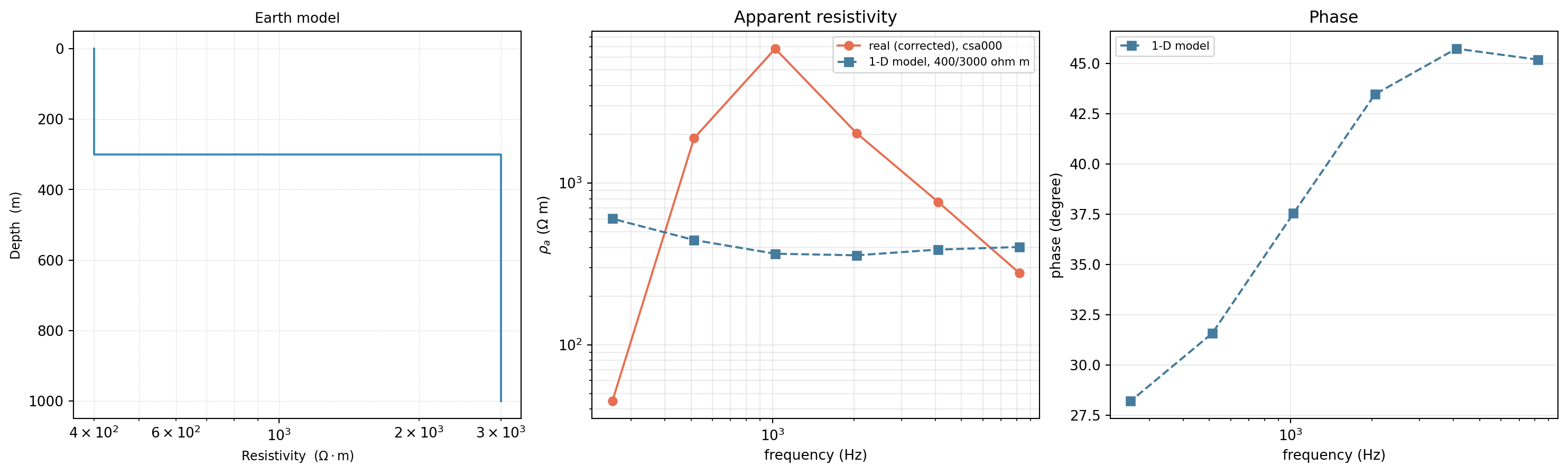
The two-layer earth model as a resistivity-depth staircase, next to real corrected apparent resistivity and the 1-D model's phase at station csa000. — Left: the model itself, `plot_model_1d()`’s own resistivity-depth staircase – 400 \(\Omega\cdot\)m to 300 m, then 3000 \(\Omega\cdot\)m below, nothing more. Middle: that model’s apparent resistivity against the real corrected sounding. Right: the model’s phase (no real phase overlay – the correction was defined on \(\rho_a\) alone). The model sits close to the real curve at the two ends of the band and misses the middle peak entirely.#

That mismatch is the finding, not a failure to fix. A single depth-only layer sequence, honestly built from this station’s own real data, already cannot explain this one sounding by itself – which is exactly the question worth asking again with a second and third station once real lateral geometry enters the picture below.

18.17.5. Choose Frequencies The Triangular Solver Can Trust#

Maxwell Analytic Benchmarks makes the general case for benchmarking a backend before trusting it. Do that here, concretely, before draping anything real over a triangular mesh. A pure half-space at the highest CSAMT frequency in this band, meshed exactly as tri_fem2d’s own benchmark recommends (\(0.04\times\) the skin depth for the near-station cell size, \(8\times\) the skin depth for the domain half-width):

>>> from pycsamt.forward.maxwell import ReceiverSet, skin_depth_m
>>> from pycsamt.forward.maxwell.contracts_tri import TriProblem
>>> from pycsamt.forward.maxwell.tri_fem2d import TriFEM2DAdapter
>>> from pycsamt.forward.maxwell.tri_mesh_gen import build_graded_tri_mesh

>>> station_x = [50.0 * i for i in range(10)]
>>> receivers = ReceiverSet([[x, 0.0] for x in station_x], [f"S{i:02d}" for i in range(10)])

>>> def half_space_check(rho, freq):
...     surface_cell_m = 0.04 * float(skin_depth_m(rho, freq))
...     half_width = 8.0 * float(skin_depth_m(rho, freq))
...     mesh = build_graded_tri_mesh(
...         (-half_width, 450.0 + half_width), (0.0, half_width), station_x,
...         surface_cell_m=surface_cell_m, growth_rate=1.3, max_cell_m=half_width / 5.0,
...     )
...     problem = TriProblem(mesh, np.full(mesh.n_triangles, 1.0 / rho), [freq], receivers)
...     result = TriFEM2DAdapter().solve(problem)
...     mu0 = 4e-7 * np.pi
...     rhoa = float(np.abs(result.impedance_v_a[0, 0, 0]) ** 2 / (mu0 * 2 * np.pi * freq))
...     return rhoa

>>> round(half_space_check(400.0, 8196.722), 1)
601.7
>>> round(half_space_check(400.0, 255.7545), 1)
433.8

A backend that is correct by definition on a uniform half-space – Maxwell Analytic Benchmarks builds exactly this case for every adapter – comes back 50% high at 8196.7 Hz and 8.5% high at 255.7545 Hz, on this survey’s own real 50 m station spacing. That is not this solver failing in general; Maxwell Adapters already calls TriFEM2DAdapter research-only for exactly this reason. Skin depth at 400 \(\Omega\cdot\)m and 8196.7 Hz is only about 111 m – barely twice the station spacing – while at 255.7545 Hz it is about 629 m, comfortably larger. The two-layer model built above, benchmarked the same way at the two lowest trustworthy frequencies:

>>> from pycsamt.forward.maxwell.benchmarks import layered_earth_impedance

>>> solver_freqs = np.array([512.8206, 255.7545])
>>> surface_cell_m = 0.04 * float(skin_depth_m(400.0, solver_freqs.max()))
>>> half_width = 8.0 * float(skin_depth_m(3000.0, solver_freqs.min()))
>>> mesh = build_graded_tri_mesh(
...     (-half_width, 450.0 + half_width), (0.0, half_width), station_x,
...     surface_cell_m=surface_cell_m, growth_rate=1.3, max_cell_m=half_width / 6.0,
... )
>>> depth = mesh.triangle_centroids_m[:, 1]
>>> resistivity = np.where(depth < 300.0, 400.0, 3000.0)
>>> problem = TriProblem(mesh, 1.0 / resistivity, list(solver_freqs), receivers)
>>> result = TriFEM2DAdapter().solve(problem)
>>> mu0 = 4e-7 * np.pi
>>> rhoa_tri = np.abs(result.impedance_v_a[0, :, 0]) ** 2 / (mu0 * 2 * np.pi * solver_freqs)
>>> np.round(rhoa_tri, 1)
array([497. , 665.4])
>>> from pycsamt.forward import LayeredModel, MT1DForward
>>> np.round(MT1DForward(solver_freqs).run(model).rho_a, 1)
array([444. , 601.4])

11.9% and 10.6% high – larger than the 5% Maxwell Analytic Benchmarks treats as a clean pass, but small enough to proceed with open eyes, and far better than the 50% seen at the top of the band. The rest of this tutorial uses only 512.8206 and 255.7545 Hz for exactly this reason: not because the real data at higher frequencies is uninteresting, but because this particular solver, on this particular station spacing, has not earned trust there yet.

18.17.6. A Real 2-D Triangular Mesh#

Drape the same two-layer guess over the line’s real station elevations – not a synthetic ridge, the actual 63.1 m of relief already read from these EDI files – and solve it at the two frequencies just cleared:

View 2-D triangular mesh source codeClick to inspect and copy the complete code

def make_2d_triangular() -> dict:
    sites, usable, elevation = _load_line()
    topo_z = elevation.max() - elevation

    surface_cell_m = 0.04 * float(skin_depth_m(RHO1, SOLVER_FREQS.max()))
    half_width = 8.0 * float(skin_depth_m(RHO2, SOLVER_FREQS.min()))
    mesh = build_graded_tri_mesh(
        (-half_width, 450.0 + half_width), (0.0, half_width), STATION_X,
        surface_cell_m=surface_cell_m, growth_rate=1.3, max_cell_m=half_width / 6.0,
        topo_x_m=STATION_X, topo_z_m=topo_z,
    )
    centroids = mesh.triangle_centroids_m
    local_terrain = np.interp(centroids[:, 0], STATION_X, topo_z)
    depth_below_terrain = centroids[:, 1] - local_terrain
    resistivity = np.where(depth_below_terrain < Z1, RHO1, RHO2)
    conductivity = 1.0 / resistivity

    station_names = [f"csa{int(x):03d}" for x in STATION_X]
    receivers = ReceiverSet(np.column_stack([STATION_X, topo_z]), station_names)
    problem = TriProblem(mesh, conductivity, list(SOLVER_FREQS), receivers)
    result = TriFEM2DAdapter().solve(problem)
    zxy = list(problem.components).index("zxy")
    rhoa_2d = np.abs(result.impedance_v_a[:, :, zxy]) ** 2 / (MU0 * 2 * np.pi * SOLVER_FREQS[None, :])

    real_rho = np.array([s.rho[:, 0, 1][[4, 5]] for s in usable])  # 512.8, 255.8 Hz columns

    fig, axes = plt.subplots(1, 2, figsize=(13, 4.8), constrained_layout=True)
    triangulation = plt.matplotlib.tri.Triangulation(mesh.nodes_m[:, 0], mesh.nodes_m[:, 1], mesh.triangles)
    im = axes[0].tripcolor(triangulation, facecolors=resistivity, cmap="turbo_r",
                            vmin=RHO1, vmax=RHO2, edgecolors="white", linewidth=0.1)
    axes[0].plot(STATION_X, topo_z, color="black", lw=1.5)
    axes[0].scatter(STATION_X, topo_z, marker="v", color="black", s=34, zorder=5)
    axes[0].set_xlim(-80, 530)
    axes[0].set_ylim(700, -80)
    axes[0].set(title="Real topography-draped triangular mesh (zoomed to the line)",
                xlabel="x (m)", ylabel="z (m)")
    fig.colorbar(im, ax=axes[0], label=r"resistivity ($\Omega$ m)")

    axes[1].plot(STATION_X, real_rho[:, 0], "o-", color="#e76f51", label="real, 512.8 Hz")
    axes[1].plot(STATION_X, real_rho[:, 1], "o--", color="#e76f51", alpha=.6, label="real, 255.8 Hz")
    axes[1].plot(STATION_X, rhoa_2d[:, 0], "s-", color="#457b9d", label="2-D model, 512.8 Hz")
    axes[1].plot(STATION_X, rhoa_2d[:, 1], "s--", color="#457b9d", alpha=.6, label="2-D model, 255.8 Hz")
    axes[1].set(title="Apparent resistivity at each real station", xlabel="station x (m)",
                ylabel=r"$\rho_a$ ($\Omega$ m)")
    axes[1].legend(fontsize=7)
    axes[1].grid(alpha=.25)
    _save(fig, "triangular_2d.png")
    return {
        "n_triangles": mesh.n_triangles,
        "rhoa_2d": rhoa_2d.tolist(),
        "real_rho": real_rho.tolist(),
        "station_names": station_names,
    }

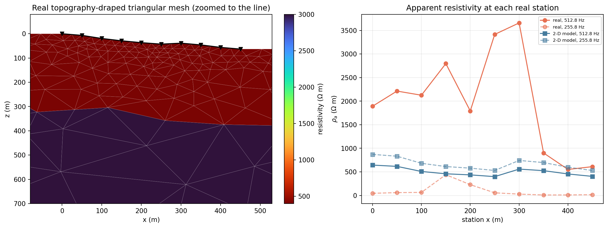
Real topography-draped triangular mesh for the Tongkeng line, and modelled versus real apparent resistivity at all ten stations. — Left: the graded triangular mesh, real station elevations followed exactly at the surface, the two-layer guess draped by depth below local terrain. Right: the draped model’s response (blue) against the real corrected data (orange) at all ten stations, both frequencies.#

The model curve moves – topography alone shifts it from about 640 \(\Omega\cdot\)m near csa000 down to about 400 near csa250, purely from following real terrain rather than a flat datum – but it moves gently, staying within roughly 400-650 \(\Omega\cdot\)m at 512.8 Hz the whole line. The real data over the same ten stations swings from about 550 to 3660 \(\Omega\cdot\)m, more than six times wider than anything topography draped over a depth-only model can produce. That is the honest answer to what a 2-D forward check adds here: real terrain explains a real, visible part of the along-line behaviour, but nowhere near enough of it – the rest has to be real lateral resistivity structure this single layered guess, draped or not, was never going to contain.

18.17.7. A 3-D Volume Mesh, Real Profile Embedded#

Tongkeng is one profile line with no real cross-line coverage, so a genuine 3-D inversion is not this survey’s to give. What is checkable honestly is narrower and still useful: embed the same real station positions, at \(y=0\), in a synthetic volume that repeats the identical two-layer structure along strike, solve it with a real compiled external solver, and confirm the production 3-D backend agrees with the 1-D analytic answer it should reduce to for a laterally uniform earth – a real, meaningful consistency check, not a demonstration for its own sake.

Before trusting any response from that volume, look at the mesh itself – the same discipline Maxwell Solver Meshes argues for on synthetic models applies just as much once real station coordinates are embedded in it.

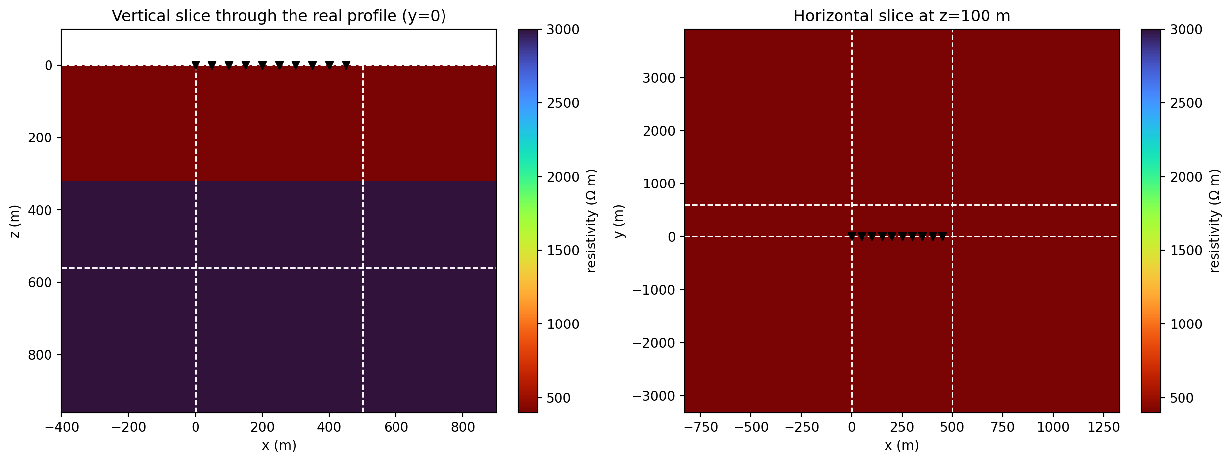
The real 3-D volume behind the response comparison below. Left: a vertical slice at \(y=0\), through the real station line (black triangles), showing the same 400 / 3000 \(\Omega\cdot\)m, 300 m-deep interface used throughout this exercise. Right: a horizontal slice at 100 m depth, showing the line’s real along-strike extent against the padded volume around it. Dashed white lines mark the boundary between the core region – built directly from the station geometry – and the padding cells added so the volume’s edges do not leak into the solution.#

This is a 20 x 15 x 22 cell mesh (\(z \times y \times x\)), coarse by design: 14 real earth layers at 40 m plus padding, enough to check that the production solver reduces to the 1-D answer for a laterally uniform earth, not to resolve fine structure. The mesh’s own quality diagnostics say so honestly – a cell-width ratio of 24.1 (target under 20) and only 2.2 core cells per minimum skin depth (target 4) are both flagged as advisory warnings, the same kind of self-reported limitation the triangular mesh carried into the previous section.

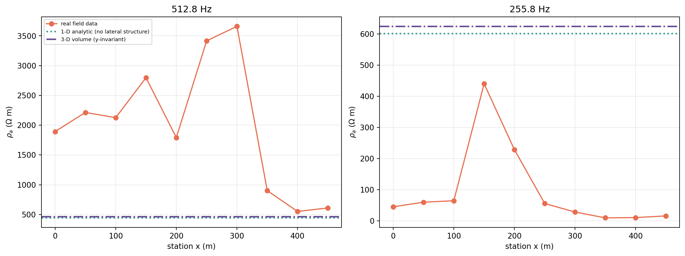
Real data (orange) at all ten stations against two dimension-blind predictions: the 1-D analytic answer for the two-layer model (teal, dotted) and the 3-D, laterally-uniform volume solved with a real compiled Mod3DMT (purple, dash-dot). The two flat lines sit close together and close to the 1-D value already computed above – and both sit far below almost every real station.#

ModEm3DAdapter’s response is 467.5 and 624.1 \(\Omega\cdot\)m at the two frequencies – within about 5% of the exact 1-D analytic answer (444.0, 601.4), a production solver reproducing plane-layered physics far more tightly than the research-grade triangular solver managed on the same model two sections ago. That agreement is the useful result on its own: it confirms the 3-D mesh and solver are set up correctly, entirely independent of whether this particular earth model explains Tongkeng. It does not. Every real station away from the flattest stretch of the line sits well above both flat predictions, several of them by a factor of five or more – the same conclusion the 2-D section reached from a different direction, now confirmed from a third, independently validated solver rather than resting on one triangular mesh’s word alone.

18.17.8. What Each Dimension Added#

Step	What it answered	What it could not
1-D	A depth-only guess, honestly built from one real sounding’s rise from 277 to a few thousand \(\Omega\cdot\)m	The real mid-band peak at that same station, or anything about the other nine
2-D triangular	How much of the real along-line swing is explained by real topography alone (some, at 512.8 Hz roughly a 250 \(\Omega\cdot\)m range out of a real 3100 range)	The remaining, much larger swing – real lateral resistivity structure this exercise never modelled
3-D volume	Whether a production solver reproduces the exact 1-D answer for a laterally uniform earth (yes, within about 5%)	Genuine 3-D structure – this survey has no cross-line data to constrain it honestly

None of the three steps produces a model of Tongkeng worth reporting – that was never the goal. Each one produces a specific, falsifiable statement about what a specific class of assumption can and cannot explain on this real line, checked against this line’s own real data rather than assumed from the method’s name.

18.17.9. Troubleshooting#

bostick_depth(sites) returns rho_a_ohmm == 0.0 for every row: Expected for a single-component (Ex-Hy only) survey. Its geometric-mean formula needs both \(Z_{xy}\) and \(Z_{yx}\); use bostick_depth_from_rho() directly on site.rho[:, 0, 1] instead.
TriFEM2DAdapter’s half-space check is far more than 5% off: Expected at CSAMT frequencies close to or above the point where skin depth approaches the real station spacing. Drop to lower frequencies in the trustworthy band, or accept a larger, explicitly stated error bar before using the result quantitatively.
ModEm3DAdapter raises “requires the mesh’s top z edge at 0”: Build the 3-D MeshDesign with air_layers=0 for this adapter specifically – ModEM writes its own air layers and refuses a mesh that already has some, exactly as Maxwell Solver Meshes describes for the rectilinear mesh contract in general.

18.17.10. See Also#

Map Groundwater Geology From CSAMT: The full near-field correction derivation for this exact survey, and the AI-inversion/groundwater-mapping application this tutorial deliberately does not repeat.
Field Zones: Near, Transition, And Far Field: Field-zone classification and the near-field correction formula this tutorial reuses rather than re-derives.
Maxwell Solver Meshes: The synthetic, systematically-varied companion to this tutorial’s real 2-D and 3-D meshes – padding, skin-depth resolution, and mesh convergence in full.
Maxwell Analytic Benchmarks: The general case for benchmarking a backend before trusting it, applied concretely to a real survey’s own station spacing here.
Maxwell Adapters: Full adapter-by-adapter coverage, including why TriFEM2DAdapter is research-only and ModEm3DAdapter is production-grade.
Prepare A MARE2DEM Inversion: Builds a triangular mesh for a real profile through the classical MARE2DEM route instead – native .poly files and an external executable, rather than this tutorial’s in-process solve.