
18.9. Stratagem Field Data To Occam2D Inversion#
Field-to-Inversion Case Study takes a real Stratagem field delivery (K2, 87 stations) from raw hardware output through coordinate injection, static-shift correction, frequency filtering, noise removal, and export – and stops there, handing off to “any of the inversion backends this documentation covers separately.” This tutorial is that next step, on a second, independent real line: Dafang line 5, 21 surviving stations over a 400 m profile. It goes all the way through a real, compiled Occam2D inversion, and adds one thing the K2 walkthrough does not have: an independent second correction of the same physical line (by an earlier, unrelated tool) to cross-check pyCSAMT’s own output against.
18.9.1. What You Will Learn#
After this tutorial you should be able to:
load a raw Stratagem WinGLink export and its matching hardware delivery, and recognise a real per-station export gap when one exists;
inject real coordinates with
CoordinateInjector, including the column-naming quirk this delivery shares with K2;sanity-check a correction pipeline’s output against an independent tool’s correction of the same real stations;
run
StaticShiftCorrector,FrequencyFilter, andNoiseRemoverend to end and read their real output honestly, including benign log noise this dataset triggers that K2 does not;build native Occam2D input files with
pycsamt.models.occam2d.InputBuilderfrom stratagem-corrected EDI, following the same recipe as Prepare an Occam2D Inversion;run a real, locally-compiled Occam2D inversion and read an honest, non-perfectly-converged result rather than a cherry-picked one.
18.9.2. Starting Point#
The bundled data lives under data/stratagem/Dafang/ –
df5-edi/ (WinGLink export, placeholder coordinates), df5-hx/ (raw
Stratagem hardware delivery, all three components), df5-coords.csv
(reconciled station coordinates), and df5-watex-edi/ /
df5-watex-edi-processed/ (an independent correction of the same line
by an earlier tool, used later for cross-validation). See
data/stratagem/Dafang/README.md for exactly what each file is and how
it was curated.
Every path below is a plain string. To run this tutorial against a
different Stratagem line, replace the four data/stratagem/Dafang/...
paths with your own WinGLink export directory, raw hardware directory,
and coordinate table – nothing else in this tutorial is Dafang-specific.
18.9.3. Loading Raw Stratagem Data#
EDIBatch loads the WinGLink export exactly as
delivered. Every station reports the same placeholder location – a
finite, valid-looking (0, 0) that nothing downstream will complain
about on its own:
>>> from pycsamt.stratagem import EDIBatch

>>> batch = EDIBatch("data/stratagem/Dafang/df5-edi").fit()
>>> len(batch.edi_objects_)
21
>>> uninjected_latlon = [
...     (e.get_section("head").Location.latitude, e.get_section("head").Location.longitude)
...     for e in batch.edi_objects_
... ]
>>> set(uninjected_latlon)
{(0.0, 0.0)}
Only 21 objects load, not 22. The raw hardware delivery at
df5-hx/ genuinely has all 22 stations’ X/Y/Z files;
ZDF5X019.edi is simply absent from the WinGLink export – a real gap
in that export, not a filtering step pyCSAMT applied:
>>> stations = sorted(e.station for e in batch.edi_objects_)
>>> "ZDF5X019" in stations
False
>>> stations[:3], stations[-3:]
(['ZDF5X001', 'ZDF5X002', 'ZDF5X003'], ['ZDF5X020', 'ZDF5X021', 'ZDF5X022'])
data/stratagem/Dafang/df5-coords.csv already accounts for this: its 21
rows line up with the 21 surviving stations in acquisition order, so no
row needs to be dropped before coordinate injection – unlike K2, where a
calibration shot and four checkpoint repeats had to be identified and
excluded explicitly.
18.9.4. Injecting Real Coordinates#
The easting/northing column values in df5-coords.csv are
swapped relative to their names – the same quirk Coordinate Injection
documents for K2. The column named easting (~2,850,000) is really a
Gauss-Kruger-style northing; the column named northing (~362,000) is
the real easting. epsg=32649 (UTM Zone 49N WGS84) reprojects the raw
pair for the first station to coordinates matching an independent source
– the corresponding station in df5-watex-edi/ – to six decimal
places, which is how it was confirmed rather than assumed:
>>> from pycsamt.stratagem import CoordinateInjector

>>> injector = CoordinateInjector(epsg=32649, order="forward").fit(
...     batch.edi_objects_, "data/stratagem/Dafang/df5-coords.csv",
...     easting_col="northing", northing_col="easting",
...     elev_col="elev", station_col="stations",
... )
>>> injected_latlon = [
...     (e.get_section("head").Location.latitude, e.get_section("head").Location.longitude)
...     for e in injector.edi_objects_
... ]
>>> tuple(round(v, 6) for v in injected_latlon[0])
(25.761665, 109.630124)
>>> tuple(round(v, 6) for v in injected_latlon[-1])
(25.764026, 109.633143)
Plotting both states side by side makes the placeholder-versus-real contrast impossible to miss:
>>> import matplotlib.pyplot as plt

>>> fig, (ax0, ax1) = plt.subplots(1, 2, figsize=(11, 4.4))
>>> lat0, lon0 = zip(*uninjected_latlon)
>>> _ = ax0.scatter(lon0, lat0, s=25, color="crimson")
>>> _ = ax0.set_xlim(-1, 1)
>>> _ = ax0.set_ylim(-1, 1)
>>> _ = ax0.set_title("Before injection: WinGLink placeholder")
>>> _ = ax0.set_xlabel("Longitude")
>>> _ = ax0.set_ylabel("Latitude")

>>> lat1, lon1 = zip(*injected_latlon)
>>> sc = ax1.scatter(lon1, lat1, s=25, c=range(len(lon1)), cmap="viridis")
>>> _ = ax1.set_title("After injection: real Dafang line-5 geometry")
>>> _ = ax1.set_xlabel("Longitude")
>>> _ = fig.colorbar(sc, ax=ax1, label="Station order")
>>> fig.tight_layout()
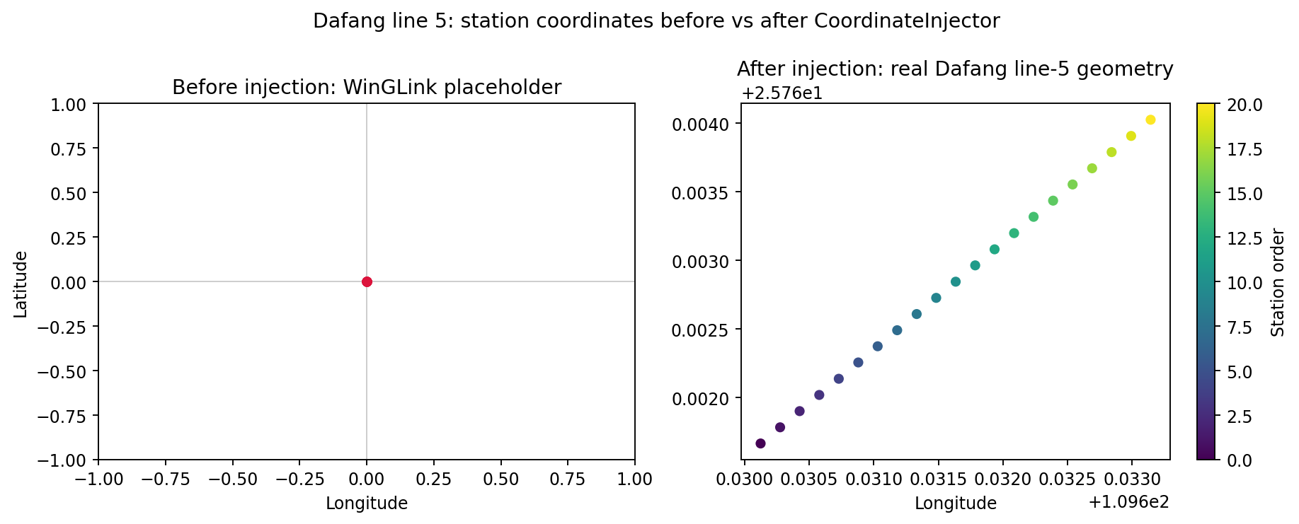
Left: all 21 stations collapsed onto (0, 0). Right: the same 21
stations spread along the real ~400 m line, coloured by acquisition
order – a short, straight profile, about a quarter of K2’s length.#
injector.edi_objects_ – the coordinate-injected objects – are what
the rest of this tutorial builds on. A deep copy taken now, before any
further correction, is what the next two sections compare against:
>>> from copy import deepcopy

>>> raw_edis = [deepcopy(e) for e in injector.edi_objects_]
18.9.5. Cross-Validating Against An Independent Tool#
Before trusting pyCSAMT’s own correction, it helps to have something
other than “the numbers changed” to check it against.
data/stratagem/Dafang/df5-watex-edi-processed/ is a real,
independently-produced correction of these same 21 physical stations, by
an earlier, unrelated tool. It is not ground truth – it used a different
static-shift algorithm and kept a different frequency subset (21 of the
original 39, versus pyCSAMT’s own selection below) – but if pyCSAMT’s
correction is doing something reasonable, the two should broadly agree on
order of magnitude and period-dependence for the same stations.
18.9.6. Static Shift, Frequency Filtering, And Noise Removal#
StaticShiftCorrector estimates
per-station correction factors from spatial neighbours (the AMA method),
then FrequencyFilter restricts every
station to a shared, hardware-validated band, and
NoiseRemover handles powerline and
outlier spikes – the same three-step chain Field-to-Inversion Case Study
runs for K2:
>>> from pycsamt.stratagem import StratagemRawReader
>>> from pycsamt.stratagem.process import StaticShiftCorrector, NoiseRemover
>>> from pycsamt.stratagem.qc import FrequencyFilter

>>> rdr = StratagemRawReader("data/stratagem/Dafang/df5-hx", component="X").fit()
>>> sc = StaticShiftCorrector(sort_by="lon").fit(injector.edi_objects_)
>>> filt = FrequencyFilter(fmin=10.0, fmax=10000.0).fit(sc.edi_objects_, raw_reader=rdr)
>>> nr = NoiseRemover(mains_hz=50.0).fit(filt.edi_objects_)
>>> final_edis = nr.edi_objects_
>>> len(raw_edis), len(final_edis)
(21, 21)
Unlike K2, this line’s raw hardware capture has a genuinely different
number of frequencies at every station (39, 38, 36, …) rather than one
fixed table shared by all stations. That is real and harmless, but it
means estimate_ss_ama()’s internal spatial
window – which briefly compares differently-sized frequency arrays while
searching for neighbours – logs a burst of ERROR-level “Failed to
compute rho/phi after setting Z” lines during StaticShiftCorrector.fit().
They look alarming but are non-fatal: every one is caught internally, and
the actual correction factors and corrected data are unaffected, which is
worth confirming directly rather than trusting the log level:
>>> sc.factors_[["station", "fac_z", "n_used"]].to_string(index=False)
' station    fac_z  n_used\nZDF5X001 0.786788      15\nZDF5X002 0.930320      14\nZDF5X003 1.281865      10\nZDF5X004 0.719025       9\nZDF5X005 1.033986       8\nZDF5X006 0.928252      10\nZDF5X007 1.289578      12\nZDF5X008 0.681909       5\nZDF5X009 1.770830      10\nZDF5X010 0.922494      17\nZDF5X011 0.710860      20\nZDF5X012 0.601690      16\nZDF5X013 1.198126      14\nZDF5X014 0.864620      14\nZDF5X015 1.403834      21\nZDF5X016 0.756371      14\nZDF5X017 6.290689      10\nZDF5X018 1.163751      23\nZDF5X020 0.727790      18\nZDF5X021 1.148781      11\nZDF5X022 0.805522      20'

>>> import numpy as np
>>> total_nan = sum(int(np.isnan(e.Z.z).sum()) for e in final_edis)
>>> total_nan
0
Station ZDF5X017 stands out immediately – fac_z=6.29 is far above
every other station’s factor of roughly 0.6-1.8, the same kind of single
strong outlier K2’s own outlier (station 61, fac_z≈93) was. Now the
independent-tool comparison from the previous section becomes concrete:
plot pyCSAMT’s corrected curve for ZDF5X001, ZDF5X011, and this
outlier ZDF5X017 against the WATEX-processed curve for the same three
physical stations (S00, S10, S20 in WATEX’s own naming, same
acquisition order). A second, different kind of check is worth running
alongside it: smooth_logfreq() is
pyCSAMT’s own in-house log-frequency smoother (a triangular kernel by
default), not an independent tool – it cannot confirm the correction is
right the way the WATEX comparison can, but it shows whether the
corrected curve’s station-to-station scatter is dominated by real
structure or by point-to-point noise that a smoother collapses away:
>>> from pycsamt.emtools.remove_noise import smooth_logfreq

>>> wx = EDIBatch("data/stratagem/Dafang/df5-watex-edi-processed").fit()
>>> smoothed = list(smooth_logfreq(final_edis, win=5, kind="tri", also="z", inplace=False, verbose=0))
>>> pick_idx = [0, 10, 20]
Two rows, three stations each – the top row against WATEX, the bottom row against pyCSAMT’s own smoother:
>>> fig, axes = plt.subplots(2, 3, figsize=(13, 8.0))
>>> for col, i in enumerate(pick_idx):
...     ed = final_edis[i]
...     ew = wx.edi_objects_[i]
...     per = 1.0 / ed.Z.freq
...     perw = 1.0 / ew.Z.freq
...     ax = axes[0, col]
...     _ = ax.loglog(per, ed.Z.res_xy, "o-", ms=3, lw=1, color="#d62728", label="pycsamt corrected")
...     _ = ax.loglog(perw, ew.Z.res_xy, "s--", ms=3, lw=1, color="#1f77b4", label="WATEX processed")
...     _ = ax.set_title(f"{ed.station} / {ew.station}")
...     es = smoothed[i]
...     pers = 1.0 / es.freq
...     ax2 = axes[1, col]
...     _ = ax2.loglog(per, ed.Z.res_xy, "o-", ms=3, lw=1, color="#d62728", label="pycsamt corrected")
...     _ = ax2.loglog(pers, es.rho[:, 0, 1], "^-", ms=3, lw=1.2, color="#2ca02c", label="pycsamt smoothed")
...     _ = ax2.set_xlabel("Period (s)")
...     _ = ax2.set_title(f"{ed.station} (smooth_logfreq)")
...
>>> _ = axes[0, 0].set_ylabel(r"$\rho_{a,xy}$ ($\Omega\cdot$m)")
>>> _ = axes[0, 0].legend(fontsize=8)
>>> _ = axes[1, 0].set_ylabel(r"$\rho_{a,xy}$ ($\Omega\cdot$m)")
>>> _ = axes[1, 0].legend(fontsize=8)
>>> fig.tight_layout()
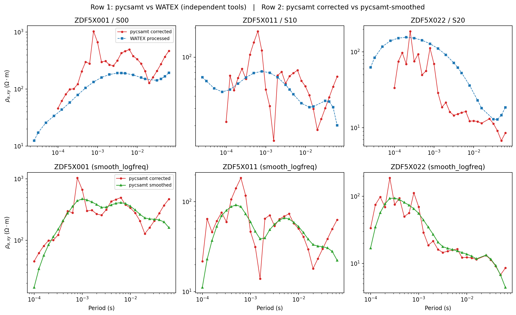
Top row: two independent tools, two different static-shift algorithms,
two different frequency selections – and both land within roughly a
factor of 2-3 of each other in the well-covered mid-period range for
all three stations, with the same broad rise-then-plateau shape. They
are not identical – pyCSAMT’s curve is visibly noisier at the short-
and long-period ends where fewer frequencies survive filtering, and
station 022’s two curves diverge more than the other two at long
periods. Bottom row: smooth_logfreq tracks the corrected curve’s
overall shape closely while damping exactly the kind of point-to-point
spikes visible in the top row – confirming those spikes are
high-frequency scatter riding on a smoother real trend, not evidence
that the underlying correction is wrong. Treat both rows as
plausibility checks on the general size and shape of the correction,
not proof that any one curve’s absolute values are exactly right.#
18.9.7. Station Map And Pseudosections#
pycsamt.map.plot_station_map() reads the corrected EDI list
directly:
>>> from pycsamt.map import StationMapOptions, plot_station_map

>>> fig = plot_station_map(
...     final_edis,
...     options=StationMapOptions(
...         overlay="rho", frequency=1000.0, frequency_tolerance=200.0,
...         component="xy", backend="matplotlib", show_labels=False,
...         show_profiles=True, cmap="viridis",
...         title="Dafang line 5: apparent resistivity at 1000 Hz",
...     ),
... )
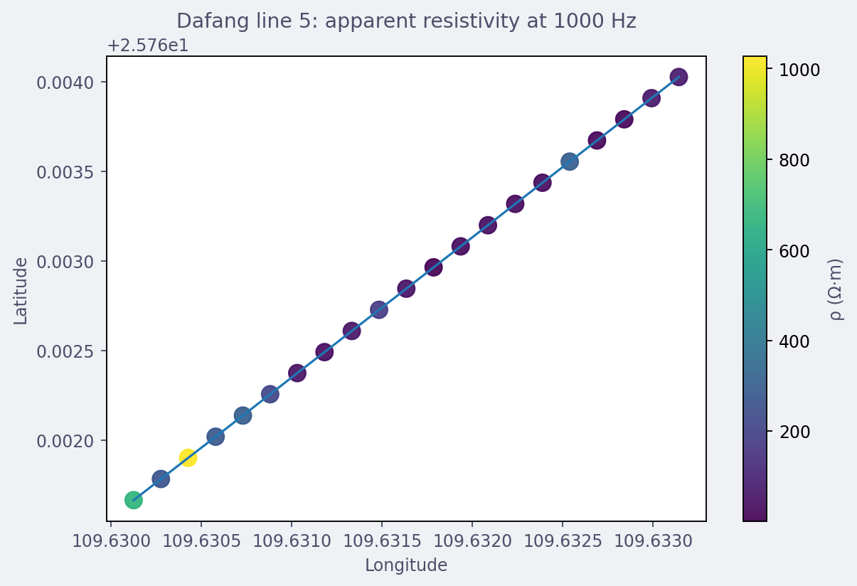
A short, straight 400 m line – more resistive (yellow-green) toward the western end, more conductive (dark purple) toward the middle and east.#
The same before/after comparison K2’s tutorial makes with
plot_pseudosection() carries over directly:
>>> from pycsamt.map import ProfileMapOptions, plot_pseudosection

>>> pseudo_opts = dict(component="xy", components=("xy",), x_axis="station", backend="matplotlib", log_rho=True)
>>> fig_final = plot_pseudosection(final_edis, options=ProfileMapOptions(**pseudo_opts))
>>> _ = fig_final.axes[0].set_title("After static shift, frequency filtering, and noise removal")
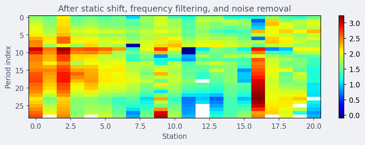
Station 17’s outlier correction shows up here too, as the isolated warm-coloured column near the middle of the line where the raw panel (not shown) reads noticeably darker.#
18.9.8. Quality Control And Export#
The same two checks Field-to-Inversion Case Study runs for K2 – no unresolved gaps, and reasonable per-station frequency coverage – matter here too:
>>> total_cells = sum(e.Z.z.size for e in final_edis)
>>> total_nan, total_cells
(0, 2392)

>>> n_freqs = [e.Z.z.shape[0] for e in final_edis]
>>> min(n_freqs), max(n_freqs), int(np.median(n_freqs))
(24, 29, 29)
The spread is worth seeing as a distribution, not just three numbers:
>>> fig, ax = plt.subplots(figsize=(6.5, 3.6))
>>> _ = ax.hist(n_freqs, bins=range(min(n_freqs), max(n_freqs) + 2), color="#3b6fa0", edgecolor="white")
>>> _ = ax.set_xlabel("Usable frequencies per station (after filtering)")
>>> _ = ax.set_ylabel("Station count")
>>> _ = ax.set_title("Dafang line 5 -- final per-station frequency coverage")
>>> fig.tight_layout()
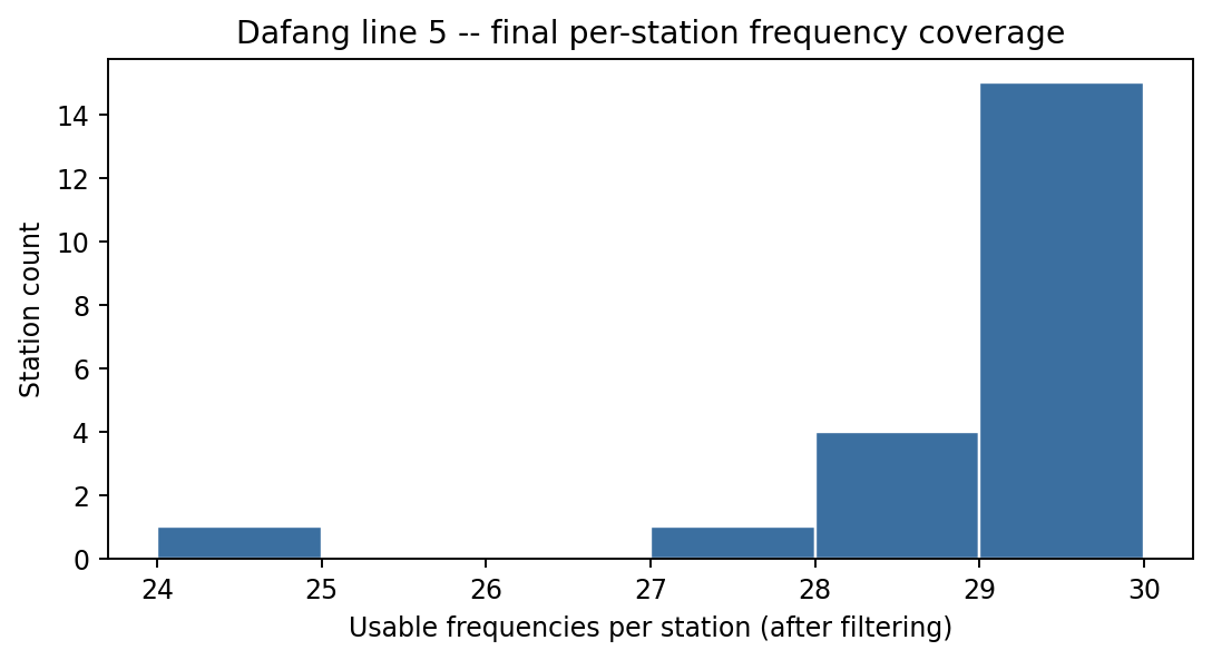
Tighter and more uniform than K2’s own 8-29 spread – 15 of 21 stations here keep the full 29-frequency band, with a short tail down to 24.#
Writing the corrected batch out is the same call as K2’s own export step:
>>> from pycsamt.stratagem.rename import EDIWriter
>>> from tempfile import TemporaryDirectory

>>> with TemporaryDirectory() as out:
...     wr = EDIWriter().fit(final_edis, out)
...     wr.n_written_
...
21
18.9.9. Preparing And Running An Occam2D Inversion#
From here, final_edis is ordinary corrected EDI input – the exact
starting point Prepare an Occam2D Inversion assumes. This section
follows that same recipe directly against the Dafang data rather than
re-explaining it. Dafang line 5 is a scalar CSAMT line (dominant Ex-Hy
component, the same configuration Field Zones: Near, Transition, And Far Field and
Field-to-Inversion Case Study describe for K2), so a TE-only
build is the appropriate first trial:
>>> from pathlib import Path
>>> from pycsamt.models.occam2d import OccamConfig, InputBuilder

>>> run_root = Path("runs")
>>> run_root.mkdir(exist_ok=True)
>>> workdir = run_root / "dafang_line5_occam2d"
>>> workdir.mkdir(parents=True, exist_ok=True)

>>> cfg = OccamConfig(
...     modes=["TE"],
...     freq_min=10.0,
...     freq_max=10000.0,
...     error_floor_rho=0.15,
...     error_floor_phase=2.0,
...     n_layers=28,
...     n_airlayers=0,
...     cell_size_horizontal=20.0,
...     cell_size_vertical_top=8.0,
...     depth_scale=1.15,
...     target_misfit=1.5,
...     max_iterations=60,
...     initial_rho=100.0,
... )
>>> builder = InputBuilder(final_edis, workdir=workdir, config=cfg, verbose=0)
>>> _ = builder.build(title="Dafang line 5 pyCSAMT v2 Occam2D preparation")
>>> print(builder.summary())
InputBuilder summary
  workdir   : runs\dafang_line5_occam2d
  sites     : 21
  freqs     : 29
  data pts  : 1196
  mesh      : 34 x 28 cells
  params    : 336
  modes     : ['TE']
n_airlayers=0 here is deliberate, not a default left untouched: the
real, compiled Occam2D solver manages its own air padding internally and
does not expect the mesh file to carry extra air rows at all. Requesting
air layers through OccamConfig produces
input files that look complete but that a real Fortran Occam2D refuses
to read (see the note below); 0 is the value that actually works
against the real solver.
detect_file_type confirms the
four files are what they claim to be before anything is sent to a solver:
>>> from pycsamt.models.occam2d.validation import detect_file_type

>>> for filename in (cfg.data_file, cfg.mesh_file, cfg.model_file, cfg.startup_file):
...     path = workdir / filename
...     print(path.name, "->", detect_file_type(path))
...
OccamDataFile.dat -> data
Occam2DMesh -> mesh
Occam2DModel -> model
Startup -> startup
Note
Building these input files does not itself require a Fortran compiler.
Actually running the solver does – Run Classical Inversions: Occam2D, ModEM, and MARE2DEM
covers discover_binary() and
compile() in full, including
why most environments should treat the run step as a dry-run command
rather than something to execute inline. This tutorial’s own run below
used a real local gfortran/make toolchain – the first time, in
the course of writing it, that a genuinely compiled Occam2D binary had
been run against pyCSAMT-built input files end to end. That surfaced
two real, now-fixed bugs that every prior dry-run example could not
have caught: compile() was
looking for a binary named Occam2D when Windows/MinGW toolchains
produce Occam2D.exe, and OccamMesh
was writing the air-layer count into the mesh file’s fixed-resistivity
field, corrupting every field after it for a real Fortran reader. Both
are fixed as of this tutorial; n_airlayers=0 above works around the
second issue’s remaining root cause – pyCSAMT’s mesh/model coupling
does not yet offer a working non-zero air-layer count against the real
solver.
Running it end to end, with a real gfortran/make toolchain on
PATH:
>>> from pycsamt.models.occam2d import OccamRunner

>>> runner = OccamRunner(workdir=workdir, verbose=0)
>>> exit_code = runner.run(max_iter=60, target_misfit=1.5, auto_compile=True)
>>> exit_code
0
18.9.10. Interpreting The Inversion#
Finishing without an error is not the same as converging.
InversionResult reads the same honesty
Run Classical Inversions: Occam2D, ModEM, and MARE2DEM insists on for every backend – check the
RMS history, not just whether loading succeeded:
>>> from pycsamt.models.occam2d import InversionResult

>>> res = InversionResult(workdir, iteration=60)
>>> print(res.summary())
InversionResult
  workdir    : runs\dafang_line5_occam2d
  iterations : 61
  final RMS  : 11.2020
  converged  : False
converged: False is the number that matters; the misfit-by-iteration
plot shows exactly how it got stuck:
>>> fig = res.plot_misfit()
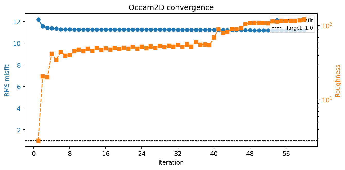
RMS drops from 12.2 to about 11.2 within the first handful of
iterations, then stalls there for the rest of the run while roughness
keeps climbing – the model getting more structured without actually
fitting the data any better, the same stalling pattern
Run Classical Inversions: Occam2D, ModEM, and MARE2DEM documents for its own bundled ModEM
sample (RMS 3.52 to 3.06 over 74 iterations, also “No”). A target
misfit of 1.5 was never realistic for a first TE-only trial with
error_floor_rho=0.15 on 21 real, noisy, static-shift-corrected
stations – tightening error floors or switching to a joint TE/TM
build (once a usable YX/TM signal is confirmed) are the next
parameters to revisit, not something this tutorial tunes to a clean
RMS=1 finish.#
>>> fig2 = res.plot_model(depth_max=600.0, rho_min=10.0, rho_max=3000.0, figsize=(9, 5))
>>> ax = fig2.axes[0]
>>> _ = ax.set_xlim(-0.05, 0.45)
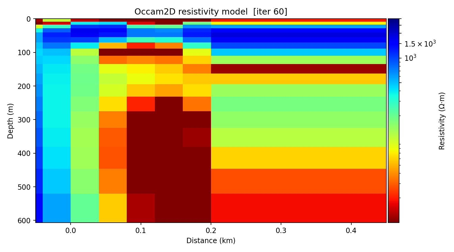
A resistive body under the western third of the line (blue, roughly 0-150 m station distance) against a more layered, moderately conductive structure under the rest of the profile – broad, smooth features consistent with a model that stalled well short of fitting fine-scale structure in the data. Read this as “what an under-converged first trial looks like,” not as a finished interpretation: with a stalled RMS of 11.2, specific resistivity values and boundary depths here are much less trustworthy than the coarse west-versus-rest contrast itself.#
18.9.11. Reusing This With Your Own Data#
Every step above generalises directly to another Stratagem line:
Point
EDIBatchat your own WinGLink export directory instead ofdata/stratagem/Dafang/df5-edi.Point
StratagemRawReaderat your own raw hardware directory instead ofdata/stratagem/Dafang/df5-hx.Build (or receive) your own coordinate table in place of
df5-coords.csv. Check the same two things this tutorial had to check: does the EDI count match the coordinate-table row count after dropping any calibration/checkpoint rows, and areeasting/northingactually in the columns their names claim?Confirm the correct EPSG the same way this tutorial did – reproject one station and compare against any independent coordinate you already trust, rather than assuming a default.
Keep or drop the WATEX-style cross-validation section depending on whether an independent correction of the same line is available; it is optional, not part of the pipeline itself.
Everything from static-shift correction onward – correction, QC, export, Occam2D preparation, and the run itself – is identical code, unchanged.
18.9.12. See Also#
- Field-to-Inversion Case Study
The K2 field-to-export case study this tutorial continues from, including the coordinate-reconciliation and outlier-correction patterns reused here.
- Prepare an Occam2D Inversion
The full
OccamConfig/InputBuilderwalkthrough this tutorial’s inversion section follows directly.- Run Classical Inversions: Occam2D, ModEM, and MARE2DEM
Compiling and running Occam2D, ModEM, and MARE2DEM in depth, including why most environments should treat the run step as a dry run.
- Field Zones: Near, Transition, And Far Field
Background on scalar (single-off-diagonal-component) CSAMT lines like K2 and Dafang line 5.
data/stratagem/Dafang/README.mdFull provenance, the WinGLink station-19 gap, the coordinate-column quirk, and the two real pyCSAMT bugs this tutorial’s real Occam2D run found and fixed.