6.3.3. Canonical data contracts#

Every stage in Architecture roadmap’s package map — a geological prior, a 2-D or 3-D Maxwell forward solve, an injected noise model, a training loss, a validation report — needs to agree on what “the data” actually is: which axis is the station, which is the frequency, whether an entry is missing or merely zero, and which sign convention the complex impedance uses. pycsamt.ai.data is where that agreement is written down once, as code, rather than assumed silently in every consumer. Its central object, SurveyData — the shared vocabulary of Correlated geological priors, Domain-gap and noise simulation, 2-D Maxwell training-data generation, 3-D Maxwell training-data generation, Loss functions for scientific inversion, and Recovery, residual, and OOD diagnostics — stores the impedance tensor in a fixed (station, frequency, component) axis order. That sounds almost too small to matter, but swapping two axes of the same rank is exactly the kind of error that produces a runnable, plausible-looking result instead of a crash — the actual failure mode this contract exists to close off.

Reach for SurveyData any time survey observations cross a function boundary in the AI-inversion stack: converting real EDI data into training features, generating a synthetic response to compare against a solver’s prediction, or handing a batch of stations to a loss function. It is not a replacement for pycsamt.site.Sites or the pandas-heavy diagnostics in pycsamt.emtools — those remain the right tools for exploratory QC. SurveyData is deliberately downstream of that: a dependency-light, NumPy-only, validated array container that every later numeric stage can trust without re-checking.

6.3.3.1. Building a survey#

The constructor accepts plain arrays directly, which is the natural way to build a survey by hand — in a test, in a small worked example, or from an in-memory synthetic response:

>>> import numpy as np
>>> from pycsamt.ai.data import SurveyData

>>> z = np.ones((2, 3, 2), dtype=complex) * (1 + 2j)
>>> survey = SurveyData(
...     impedance=z,
...     frequencies_hz=[100.0, 10.0, 1.0],
...     station_names=["S01", "S02"],
...     components=["xy", "yx"],
...     coordinates_m=[[0.0, 0.0], [100.0, 0.0]],
...     crs="EPSG:32630",
... )
>>> survey.shape
(2, 3, 2)
>>> survey.frequency_order
'descending'

A two-column coordinates_m is accepted and silently expanded with an unknown (NaN) elevation column, so callers who genuinely have no elevation are not forced to invent one.

Optional tipper data follow a separate but equally explicit contract: tipper, tipper_error, and tipper_valid have shape (station, frequency, 2), with the last axis ordered as \(T_x,T_y\). Tipper errors or masks cannot be supplied without tipper values. As with impedance, non-finite values and non-positive declared errors invalidate an observation; they are never converted into zero induction arrows. Keeping tipper outside the impedance component axis prevents a four-component tensor from being confused with two magnetic transfer functions.

Real field data rarely arrives already shaped this way. The practical entry point is pycsamt.ai.domain_gap.survey_fit.survey_data_from_sites(), which bridges anything pycsamt.emtools._core.ensure_sites() already accepts — a directory of EDI files, a loaded Sites collection, an APISurvey — into a canonical SurveyData, using the full xx, xy, yx, yy component set:

>>> from pycsamt.emtools._core import ensure_sites
>>> from pycsamt.ai.domain_gap import survey_data_from_sites

>>> sites = ensure_sites(
...     "data/AMT/WILLY_data/L18PLT", recursive=True, verbose=0
... )
>>> field = survey_data_from_sites(sites, recursive=False, verbose=0)
>>> field.shape
(28, 53, 4)
>>> field.summary()["coverage"]
1.0
>>> field.summary()["frequency_range_hz"]
[1.008, 10400.0]

This bridge performs no frequency interpolation across stations: if two stations were sampled on different grids, construction raises rather than quietly reconciling them, because a survey-matched frequency selector is a scientific decision this package refuses to make on a caller’s behalf.

6.3.3.2. The 3-D Maxwell dataset contract#

The completed 3-D path uses the same SurveyData response contract, but it must preserve more than the response tensor. A Maxwell3DSample binds one converged survey to the true (z, y, x) resistivity volume that generated it, the realization ID and seed, the solver problem hash, mesh-cell count, residual, and runtime. Maxwell3DDataset then binds all samples to one geology grid, a realization-level split, a manifest, and the IDs of rejected solves.

The following small run exercises that complete route rather than constructing shapes by hand. Its three realizations are intentionally tiny enough for a documentation check; they are not a useful training corpus:

>>> from pycsamt.ai.geology import GeologyGrid
>>> from pycsamt.ai.training.dataset3d import (
...     Maxwell3DDatasetConfig, generate_3d_maxwell_dataset,
... )
>>> grid = GeologyGrid.regular_3d(
...     nx=4, ny=4, nz=4, dx_m=250, dy_m=250, dz_m=150,
... )
>>> config = Maxwell3DDatasetConfig(
...     dataset_id="contracts-3d-smoke-v1",
...     grid=grid,
...     correlation_length_x_m=(350.0, 700.0),
...     correlation_length_y_m=(350.0, 700.0),
...     correlation_length_z_m=(100.0, 250.0),
...     frequencies_hz=[1.0],
...     station_xy_m=[[375.0, 375.0], [625.0, 625.0]],
...     n_realizations=3, seed=11, components=("zxy",),
...     mesh_safety_factor=2.0, max_mesh_cells=6000,
...     validation_fraction=1 / 3, test_fraction=1 / 3,
... )
>>> dataset = generate_3d_maxwell_dataset(config)
>>> sample = dataset.samples[0]
>>> dataset.grid.shape, sample.resistivity_ohm_m.shape
((4, 4, 4), (4, 4, 4))
>>> sample.survey.shape
(2, 1, 1)
>>> sample.survey.coordinates_m.tolist()
[[375.0, 375.0, 0.0], [625.0, 625.0, 0.0]]
>>> dataset.split.sizes, dataset.rejected
({'train': 1, 'validation': 1, 'test': 1}, ())
>>> sample.mesh_cells, dataset.manifest.sample_count
(4536, 3)
>>> len(dataset.manifest.manifest_hash)
64

The equal geology and truth-array shapes above are intentional: the sample stores truth on the geology grid. The 4536 solver cells belong to a different padded, non-uniform Maxwell mesh and are recorded as diagnostics, not reshaped into a false (z, y, x) truth array. The response shape follows the universal survey order (station, frequency, component); here that is two receivers, one frequency, and zxy only.

For realization \(r\), the contract can be summarized as

(1)#\[\mathcal R_r = \left( \rho_r[z,y,x],\; Z_r[s,f,c],\; \mathbf x_s,\; h_r,\;q_r \right),\]

where \(h_r\) is the solver problem hash and \(q_r\) contains mesh and convergence diagnostics. Equation (1) keeps geological truth, simulated observations, receiver geometry, and solver provenance attached to the same realization. A bare response array cannot provide that guarantee.

Maxwell3DDatasetConfig.to_dict() records the geology grid, station coordinates, frequency and component selections, correlation ranges, resistivity distribution, seed, split fractions, and mesh controls. The dataset manifest hashes that complete record. Consequently, changing a mesh budget or station position changes dataset identity even when the returned array shapes happen to remain equal.

Topography is a contract, not an optional picture

The current 3-D dataset generator and both exposed 3-D adapters declare no inactive-cell or topographic-mask support through this API. Receiver elevations in SurveyData.coordinates_m[:, 2] remain valuable metadata, but nonzero elevations alone do not put air cells or terrain into the Maxwell solve. Record a separate topography mapping only when the selected backend actually applies it; otherwise mark affects_forward_physics=False as AI inversion agents does.

6.3.3.3. Invalid data are never invented#

A field survey always has gaps — a saturated channel, a frequency a station never recorded, a value flagged during processing. The valid mask exists so that “missing” and “zero” are never confused, and construction computes it rather than trusting a caller’s word alone: an explicitly supplied mask is combined with a finite-value check and, when errors are declared, a positive-error check, so a NaN slipped into the impedance array cannot silently pass validation:

>>> z = np.array([[[1 + 1j], [complex(np.nan, np.nan)]]])
>>> s = SurveyData(z, [10, 1], ["S"], ["xy"], [[0, 0]])
>>> s.n_valid
1

One observation went in with a NaN, and exactly one came out valid — the second frequency is now authoritatively unusable rather than a landmine waiting in a mean or a loss term. coverage() turns this mask into a SurveyCoverage summary along every axis, which is the first thing worth checking after loading any real survey:

(2)#\[C_{\mathrm{all}}= \frac{1}{N_sN_fN_c}\sum_{s=1}^{N_s}\sum_{q=1}^{N_f} \sum_{c=1}^{N_c}v_{sqc}, \qquad C_s=\frac{1}{N_fN_c}\sum_{q,c}v_{sqc},\]

where \(v_{sqc}\in\{0,1\}\) is the authoritative validity mask, and \(N_s\), \(N_f\), and \(N_c\) are station, frequency, and component counts. Frequency and component coverage are the analogous means over their complementary axes. Equation (2) counts declared observations, not independent information: four complete tensor components can still be strongly correlated or physically unsuitable.

>>> coverage = field.coverage()
>>> round(coverage.overall, 4)
1.0
>>> coverage.by_station.min(), coverage.by_station.max()
(1.0, 1.0)

L18 happens to be unusually complete — every declared observation is finite and error-bearing, so coverage is exactly 1.0 on every axis. A survey with dropped stations or frequencies, such as the corrupted ones produced by Domain-gap and noise simulation, shows that immediately in by_station and by_frequency instead of only in a suspiciously small final sample count.

6.3.3.4. Convention is part of the data#

An impedance value is meaningless without knowing its Fourier time convention, physical units, and rotation state, so ImpedanceConvention records those explicitly rather than assuming everyone agrees. This is not decorative: Architecture roadmap’s governing 3-D equation (2) and the 2-D/3-D adapters behind it each fix one time convention per solve, and a predicted response built under exp(-iwt) compared directly against field data stored as exp(+iwt) produces a response residual that looks like a sign error in the physics rather than what it actually is — a bookkeeping mismatch. assert_compatible() is the guard that catches this before it reaches a loss or a solver:

>>> from pycsamt.ai.data.contracts import ImpedanceConvention

>>> a = field.select(stations=[0, 1])
>>> b = field.select(stations=[2, 3])
>>> rotated = SurveyData(
...     b.impedance, b.frequencies_hz, b.station_names,
...     b.components, b.coordinates_m,
...     convention=ImpedanceConvention(rotation_deg=15.0),
... )
>>> a.assert_compatible(rotated)
Traceback (most recent call last):
...
ValueError: survey impedance conventions differ.

rotated is otherwise a perfectly valid survey; the only thing wrong with it is that its axes were rotated 15 degrees clockwise without the other survey’s axes moving too. Catching that with a clear error is far preferable to merge_surveys() or fit() silently pooling two surveys whose horizontal axes do not actually point the same way.

6.3.3.5. Selecting, subsetting, and merging#

select_names() is the everyday way to narrow a survey by station name, component, or a physical frequency band, independent of how frequencies happen to be stored internally:

>>> subset = field.select_names(
...     stations=field.station_names[:4],
...     components=["xy", "yx"],
...     frequency_min_hz=10.0,
...     frequency_max_hz=1000.0,
... )
>>> subset.shape
(4, 26, 2)
>>> round(float(subset.frequencies_hz.min()), 2), round(float(subset.frequencies_hz.max()), 2)
(10.16, 863.9)

The lower-level select() takes integer positions instead, which matters when composing a selection from indices computed elsewhere — a station-adjacency graph’s node order, for instance — rather than from names a person would type.

Going the other way, merge_surveys() concatenates compatible surveys along the station axis, refusing to proceed unless every survey agrees on frequencies, components, CRS, and convention first:

>>> from pycsamt.ai.data.contracts import merge_surveys

>>> merged = merge_surveys([a, b])
>>> merged.station_names
('18-001A', '18-002U', '18-003A', '18-004A')
>>> merged.shape
(4, 53, 4)

This is the operation behind combining several acquisition batches or survey lines into one dataset for training or validation, and it performs no interpolation, projection, or rotation of its own — those remain explicit steps a caller must have already completed, precisely so that a merge cannot quietly average away a real, meaningful difference between two lines.

6.3.3.6. Fitting a normalizer once, reusing it everywhere#

Neural networks train far better on standardized inputs, but how that standardization is computed is a scientific choice, not a mechanical one: fit it on the wrong data and every later prediction inherits that mistake invisibly. ComplexZScore standardizes the real and imaginary impedance channels independently, per frequency and per component, from training data only, and then stores that state so validation, test, and field data are transformed with the exact same numbers rather than refit each time. For one channel \(x_i\) (a real or imaginary part) at a fixed frequency and component, with fitting weight \(w_i\) — uniformly one per valid observation, or the inverse-variance \(1/\sigma_i^2\) from a declared impedance_error when weighting="inverse_variance" — the fitted statistics and the standardized value are

(3)#\[\bar x = \frac{\sum_i w_i x_i}{\sum_i w_i}, \qquad s = \max\!\left(\sqrt{\frac{\sum_i w_i (x_i-\bar x)^2} {\sum_i w_i - \mathrm{ddof}}},\ \varepsilon\right), \qquad z_i = \frac{x_i-\bar x}{s}.\]

The \(\varepsilon\) floor in equation (3) keeps a channel that happens to be constant across the training set from producing a division by zero, and ddof behaves like NumPy’s usual delta-degrees-of-freedom correction (it must be zero under inverse-variance weighting, where the weighted second moment already plays that role). Fitting and applying this to the real L18 survey shows the point of doing it per frequency rather than once globally:

>>> from pycsamt.ai.data.normalization import ComplexZScore

>>> state = ComplexZScore.fit(field)
>>> state.feature_names[:2]
('10400Hz:xx:real', '10400Hz:xx:imag')
>>> state.training_station_count
28

>>> features, mask = state.transform(field)
>>> restored = state.inverse_transform(features, valid=mask)
>>> observed = mask.all(axis=-1)
>>> float(np.max(np.abs(restored[observed] - field.impedance[observed])))
3.580361673049448e-15

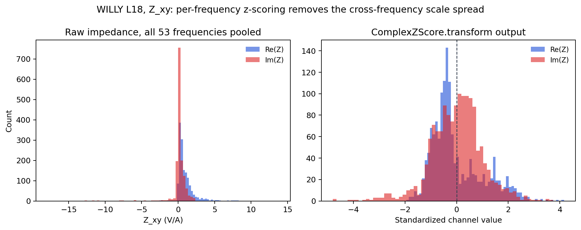
Raw versus z-scored WILLY L18 Z_xy impedance distribution — `Z_xy` pooled across all 53 frequencies spans about three orders of magnitude in the raw data (left) because low-frequency responses are physically much larger than high-frequency ones over the same layered earth — not because of any instrument fault. Standardizing per frequency (right) removes that purely spectral scale spread, leaving a distribution a network can actually learn from, while `inverse_transform()` recovers the original complex values to within floating-point error, confirmed above rather than assumed.#

That round trip is not a formality. A checkpoint saved without its exact fitted ComplexZScore state is not reproducible: the same raw impedance would standardize to different numbers under a normalizer refit on a different survey, silently changing what the network was actually trained to see. This is one instance of the broader Feature contract this whole package exists to fix in place.

For training code, keeping values and masks as unrelated arrays is still an easy way to lose their alignment. transform_survey binds them in a NormalizedSurvey, carries propagated errors when the source survey has them, labels every axis, and records the normalization state hash that produced the features:

>>> normalized = state.transform_survey(field)
>>> normalized.shape
(28, 53, 4, 2)
>>> normalized.n_valid_observations
5936
>>> flat, flat_valid = normalized.flatten()
>>> flat.shape, flat_valid.shape
((28, 424), (28, 424))
>>> normalized.errors is not None
True
>>> normalized.state_hash == state.state_hash
True

The final normalized axis is (real, imaginary), hence \(424=53\times4\times2\); n_valid_observations counts complex impedances once rather than counting both channels. Invalid entries receive a finite fill value for numerical execution, but flat_valid remains the authority for excluding them from a loss. A fill value of zero means “the training mean after normalization,” not “measured zero impedance,” and must never be used without its mask.

If \(\sigma_{Z,sqc}\) is the declared absolute complex-impedance error and \(a\in\{\Re,\Im\}\) identifies the channel, error propagation uses

(4)#\[\sigma^{\prime}_{sqca}= \frac{\sigma_{Z,sqc}}{s_{qca}},\]

with \(s_{qca}\) the fitted scale from (3). The same scalar source error is divided by different real and imaginary scales; it is not a covariance model and does not represent correlation between channels. Downstream likelihoods that need a full complex covariance must preserve that richer error model separately.

The hash is useful only if the state itself is saved. The schema-versioned dictionary is JSON serializable and round-trips to the identical digest:

>>> import json
>>> from pathlib import Path
>>> from tempfile import TemporaryDirectory

>>> with TemporaryDirectory() as directory:
...     path = Path(directory) / "normalizer.json"
...     _ = path.write_text(
...         json.dumps(state.to_dict(), indent=2), encoding="utf-8"
...     )
...     restored_state = ComplexZScore.from_dict(
...         json.loads(path.read_text(encoding="utf-8"))
...     )
...     print(restored_state.state_hash == state.state_hash)
True

Store this file beside the checkpoint and record it as an artifact in the dataset or model manifest. A matching hash proves identity of the serialized normalizer; it does not prove that the normalizer was fitted only on the training partition, so split provenance remains necessary.

6.3.3.7. Splitting realizations without leaking#

pycsamt.ai.data.splits answers a narrower, related question: once many geological realizations exist — as they do once 2-D Maxwell training-data generation or 3-D Maxwell training-data generation starts generating them — which ones may sit in training and which must be held out. The risk is the same one Training AI inversion models already states as equation (2): if two samples share a parent, a split that separates them is not a genuine test of generalization. RealizationSplit’s lineage argument is exactly that condition, made concrete and enforced in code — every realization sharing a lineage label is required to land in the same partition, checked automatically on construction by assert_no_lineage_leakage():

>>> from pycsamt.ai.data.splits import split_realizations

>>> ids = [f"r{i}" for i in range(10)]
>>> first = split_realizations(
...     ids, validation_fraction=0.2, test_fraction=0.2, seed=4
... )
>>> second = split_realizations(
...     list(reversed(ids)),
...     validation_fraction=0.2,
...     test_fraction=0.2,
...     seed=4,
... )
>>> first == second
True
>>> first.sizes
{'train': 6, 'validation': 2, 'test': 2}

Splitting is deterministic for a fixed Random seed and invariant to input enumeration, which matters in practice: a dataset regenerated in a different enumeration order — a different filesystem walk, a reshuffled manifest — must still land every realization in the same partition it did before, or a “held-out” test set silently stops being held out across reruns. Grouping several noisy variants of one clean realization under a shared lineage label keeps them together the same way:

>>> lineage = {"a-clean": "a", "a-noisy": "a", "b": "b", "c": "c"}
>>> split = split_realizations(
...     list(lineage),
...     validation_fraction=0.25,
...     test_fraction=0.25,
...     lineage=lineage,
... )
>>> split.partition("a-clean") == split.partition("a-noisy")
True

a-clean and a-noisy are two different corruption draws over the same underlying resistivity model from Domain-gap and noise simulation — a plain random split could easily put one in training and the other in test, which would let the network partly memorize that one earth model’s response rather than generalize.

When model selection requires cross-validation rather than one holdout, realization_folds() applies the same lineage rule to every test fold. Each independent lineage appears in test exactly once, while related variants remain together:

>>> from pycsamt.ai.data.splits import realization_folds

>>> lineage = {
...     "a-clean": "a", "a-noisy": "a", "b": "b", "c": "c", "d": "d"
... }
>>> folds = realization_folds(
...     list(lineage), n_splits=3, seed=7, lineage=lineage
... )
>>> [fold.sizes for fold in folds]
[{'train': 3, 'validation': 0, 'test': 2}, {'train': 3, 'validation': 0, 'test': 2}, {'train': 4, 'validation': 0, 'test': 1}]
>>> [fold.test for fold in folds]
[('a-clean', 'a-noisy'), ('c', 'd'), ('b',)]
>>> sorted(item for fold in folds for item in fold.test)
['a-clean', 'a-noisy', 'b', 'c', 'd']

Unequal fold sizes are expected when lineage groups have unequal membership; splitting a-clean from a-noisy merely to balance row counts would create lineage leakage. These folds intentionally leave validation empty. If early stopping or hyperparameter selection is performed inside each fold, create a second lineage-safe split within its training members rather than selecting on the outer test fold.

6.3.3.8. Recording what actually produced a dataset#

Everything above validates data in memory; none of it, by itself, proves that a saved dataset was produced the way its documentation claims. pycsamt.ai.data.manifest closes that gap. canonical_hash() hashes any JSON-serializable configuration deterministically — key order and whitespace never affect the digest — and DatasetManifest bundles that configuration hash together with the exact RealizationSplit used and a SHA-256 ArtifactRecord per output file, so a manifest alone is enough to detect a silently regenerated dataset, a swapped split file, or a corrupted archive:

(5)#\[h_{\mathrm{cfg}}= \operatorname{SHA256}\!\left( \operatorname{UTF8}\left[J_{\mathrm{canonical}}(\mathcal C)\right] \right),\]

where \(\mathcal C\) is the finite JSON-serializable configuration and \(J_{\mathrm{canonical}}\) recursively sorts mapping keys, removes insignificant whitespace, retains Unicode, and rejects NaN and infinity. This canonical hash makes mapping insertion order irrelevant. It does not make two scientifically equivalent configurations equal when they use different units or parameterizations; canonicalization is syntactic, not semantic.

>>> from pathlib import Path
>>> from tempfile import TemporaryDirectory
>>> from pycsamt.ai.data.manifest import DatasetManifest, ArtifactRecord
>>> from pycsamt.ai.data.splits import RealizationSplit

>>> with TemporaryDirectory() as directory:
...     root = Path(directory)
...     npz_path = field.to_npz(root / "willy_l18.npz")
...     record = ArtifactRecord.from_file(
...         npz_path, media_type="application/x-npz", role="survey"
...     )
...     manifest = DatasetManifest(
...         dataset_id="willy-l18-zscore-v1",
...         generator="pycsamt.ai.data.normalization.ComplexZScore",
...         generator_version="1.0",
...         configuration={"weighting": "uniform", "eps": 1e-8},
...         split=RealizationSplit(("willy-l18",), (), ()),
...         sample_count=field.n_stations,
...         artifacts={"willy_l18.npz": record},
...     )
...     json_path = manifest.write_json(root / "manifest.json")
...     reloaded = DatasetManifest.read_json(json_path)
...     print(reloaded.manifest_hash == manifest.manifest_hash)
...     print(manifest.verify_artifacts(root))
True
{'willy_l18.npz': True}

verify_artifacts() recomputes each recorded file’s size and digest from disk rather than trusting the manifest’s own claim about them, which is precisely what turns “a JSON file next to the dataset” into an actual integrity check: swap in a different willy_l18.npz after the fact and this call starts returning False for it, before that mismatch has any chance to reach training silently.

6.3.3.9. Accounting for every station, not just the aggregate#

coverage.overall being 1.0 on L18 is a fact about this survey, not a guarantee about the next one. A survey with dropped stations, an unstable strike, or a mismatched frequency grid needs its problems named individually, station by station — an aggregate percentage can look reassuring while hiding exactly which station is the reason it is not 1.0. audit_survey() is that per-station accounting, and it deliberately does not live in this package: strike and dimensionality come from pre2d_inversion_assessment(), and static-shift/distortion spread from fit_distortion_priors_from_sites(), both pandas-based diagnostics that pycsamt.ai.data excludes by design. It is where those heavier diagnostics and this page’s own SurveyCoverage/error-ratio numbers meet in one report.

It also does not share survey_data_from_sites()’s fail-fast stance on a mismatched frequency grid. That bridge exists to stop training from ever proceeding on inconsistent data, so it raises immediately; an audit exists to be run before that decision is made, so it never raises for the same reason — a mismatch becomes a finding in the report, not a crash that stops the audit from covering every other station:

>>> from pycsamt.ai.domain_gap import audit_survey

>>> report = audit_survey(
...     "data/AMT/WILLY_data/L18PLT", recursive=True, verbose=0
... )
>>> report.n_stations_input, report.n_stations_included
(28, 28)
>>> report.frequency_grid.matched
True
>>> round(report.error_ratio_p05, 4), round(report.error_ratio_p50, 4)
(0.0297, 0.0843)
>>> {k: round(v, 1) for k, v in report.station_spacing_m.items()}
{'min': 1.6, 'median': 98.5, 'max': 139.2}

>>> dim = report.dimensionality
>>> dim.n_samples
1484
>>> round(dim.frac_1d, 3), round(dim.frac_2d, 3), round(dim.frac_3d, 3)
(0.039, 0.104, 0.856)
>>> round(dim.strike_consensus_deg, 1), round(dim.strike_consensus_iqr_deg, 1)
(-37.6, 99.9)
>>> len(dim.stations_recommending_3d_review)
28

>>> round(report.static_shift_log10_sigma, 4)
0.2759
>>> round(report.distortion_twist_deg_sigma, 2)
26.76

L18’s own numbers make the point better than a synthetic example could: 85.6% of its 1,484 station-period samples classify as 3-D by phase-tensor skew and ellipticity, every one of its 28 stations is flagged for 3-D review, and the consensus strike carries a 99.9-degree interquartile spread — a survey this unstable in strike is not a quiet, well-behaved 1-D or 2-D line, and a training prior or a 2-D inversion built on it should say so explicitly rather than average it away. None of that is visible in coverage()’s 100% figure earlier on this page; audit_survey() is what surfaces it. Like DatasetManifest, a SurveyAuditReport supports to_dict/write_json/read_json, so an audit can be saved and diffed alongside the dataset it describes rather than only printed once and discarded.