
6.3.18. Hybrid AI and physics inversion#
Hybrid inversion is the bridge between fast learned inference and observation-specific physics refinement. The supervised model gives an initial earth estimate; the physics step then asks whether that estimate can reproduce the measured electromagnetic response under the declared solver, component, regularization, and geometry assumptions. It is not a shortcut around AI inversion validation. It is a two-stage scientific claim:
where \(\mathbf{x}\) is the feature vector or panel, \(g_\theta\) is the fitted AI inverter, \(\mathbf{m}_0\) is the Stage-1 starting model, and \(\hat{\mathbf{m}}\) is the Stage-2 refined model. A hybrid result is useful only when both stages remain visible. If the final section is shown without the initial AI estimate, the reader cannot tell whether physics refinement improved the result, merely preserved it, or moved it into a different but still non-unique model. Equation (1) also fixes the order of operations: preprocessing and AI inference precede observation-specific optimization.
Use hybrid inversion when a supervised inverter already has a validated feature contract, but field observations deserve a physical correction before interpretation. Typical cases include:
a trained
pycsamt.ai.inversion.EMInverter1Dthat gives plausible station models but leaves coherent response residuals;a 2-D section from
pycsamt.ai.inversion.EMInverter2Dthat needs station-by-station response consistency and lateral smoothing;a graph-based 3-D estimate that is useful as a spatial prior but still needs electromagnetic response checks;
a comparison scenario where a fully physics-informed run is too sensitive to naive initialization.
Do not use a hybrid workflow to rescue an AI model outside its validated domain. A Stage-2 optimizer can reduce response misfit while keeping the inversion trapped near a poor starting model, especially when bandwidth, dimensionality, or data quality differs strongly from the training distribution. This is one expression of non-uniqueness: many earth models can fit the same response within error, and a warm start can decide which basin the optimizer explores first. In that situation the hybrid result should be reported as a stress test or conditional interpretation, not as a promoted model.
6.3.18.1. Before you run it#
Hybrid inversion is most useful when a few conditions are already true. The Stage-1 model should be a validated checkpoint, not just a network that happens to load. The field or synthetic observation should pass the same preprocessing, frequency support, component order, masking, and unit conventions used during training. The Stage-2 solver should be an appropriate physical approximation for the intended use, and the regularization weights should be chosen before looking at the final section.
Treat these as pre-run gates:
the AI model was validated on a domain close to the target survey;
the input arrays satisfy the documented feature contract;
quality control has identified missing bands, outliers, static shift, and component problems;
phase tensor or other diagnostics do not contradict the assumed dimensionality;
the Stage-2 objective, weights, bounds, and stopping rule are written down;
the accepted comparison is Stage 2 against Stage 1, the baseline model, and a classical or independent reference where available.
If one of these gates fails, continue only as an exploratory run. That is not a failure of the method; it is a protection against giving a polished scientific meaning to an unsupported optimization.
6.3.18.2. The two-stage objective#
Stage 1 is a supervised inverse mapping. For a fitted AI model \(g_\theta\), the starting model is
Stage 2 starts from \(\mathbf{m}_{0,i}\) and minimizes a physics objective against the observed response. In compact form,
where inactive terms are omitted for lower-dimensional workflows. The data term compares the measured response \(\mathbf{d}^{\mathrm{obs}}\) with the response reconstructed by the forward operator:
Here \(\mathcal{M}\) is the finite data mask, \(\rho^a\) is apparent resistivity, and \(\phi\) is phase. The regularization terms encode the geometry expected from the selected parameterization. A 1-D station run usually uses vertical roughness only; a 2-D profile also uses lateral roughness; a 3-D graph workflow can penalize roughness across graph edges. The weights therefore have scientific meaning: they decide how much misfit reduction is worth compared with added structure. Thus (3) is not reproducible unless the residual definition in (4) and every active weight are reported.
The current HybridInverter1D,
HybridInverter2D, and
HybridInverter3D kernels use the more specific
unweighted objective
where a cell enters \(\mathcal M\) only when both apparent resistivity and phase are finite. Observational errors and error floors are not consumed by this kernel, so equation (7) is a recommended external validation metric, not a description of the implemented optimizer. The phase subtraction is direct rather than circular; normalize phase branches before fitting so values near a wrapping boundary do not create an artificial large residual.
The code uses means, not raw sums, for vertical and lateral differences. For an \(S\times L\) station-by-layer log-resistivity matrix \(U\),
For the quasi-3-D path, \(\mathcal J_g=\operatorname{tr} (U^T(D-A)U)/(SL)\). These normalizations matter when comparing runs with different station or layer counts. Adam optimizes log-resistivity and log-thickness through a differentiable forward model implementing a 1-D MT recursion. PyTorch and TensorFlow clip gradient norm to 5; log-thickness is clamped after every update to \([0,5]\), corresponding to 1–100,000 m. Log-resistivity has no equivalent hard clamp, so inspect it for implausible values rather than assuming positivity conversion alone makes the model geological.
The mask and weights deserve the same care as the network architecture. A typical normalized residual can be written
where \(\sigma_{ij}\) is the observational standard error or an adopted error floor. When an explicit error model is unavailable, the report should state the substitute weights. A phase residual divided by 90 degrees, a log-apparent-resistivity residual, and a statistically normalized residual are not interchangeable metrics. They answer different questions, so do not mix them without naming the residual space.
The regularization terms are usually roughness penalties. For a 2-D log-resistivity section \(u_{zk}=\log_{10}\rho_{zk}\), one possible reading is
For a graph model with edge set \(\mathcal{E}\),
where \(a_{pq}\) is an edge weight. These equations make the trade-off visible: lowering the data term by introducing sharp or isolated structure is penalized only to the degree encoded by \(\lambda_z\), \(\lambda_x\), or \(\lambda_g\). The distinction between the grid differences in (8) and graph edges in (9) matters when results are compared across dimensions.
The improvement made by Stage 2 should be measured in response space, not only by a smaller training-style loss. If \(r^{(1)}_{ij}\) and \(r^{(2)}_{ij}\) are normalized residuals for Stage 1 and Stage 2,
Positive \(\Delta_{\mathrm{NRMS}}\) means Stage 2 improved normalized response fit. It does not by itself prove geological correctness; it must be read beside model change, regularization, uncertainty, and independent evidence. Use exactly the same finite mask and error model in both terms of (10); otherwise a positive value can be created merely by discarding difficult observations.
>>> import numpy as np
>>>
>>> stage1_residual = np.array([
...     [1.4, -0.8, 0.5, 1.2],
...     [0.9, -1.1, 0.7, 1.0],
...     [1.6, -0.6, 0.4, 1.3],
... ])
>>> stage2_residual = np.array([
...     [0.8, -0.5, 0.4, 0.7],
...     [0.6, -0.7, 0.5, 0.6],
...     [0.9, -0.4, 0.3, 0.8],
... ])
>>> nrms1 = np.sqrt(np.mean(stage1_residual ** 2))
>>> nrms2 = np.sqrt(np.mean(stage2_residual ** 2))
>>> improvement = nrms1 - nrms2
>>> print("Stage-1 NRMS:", round(float(nrms1), 3))
Stage-1 NRMS: 1.023
>>> print("Stage-2 NRMS:", round(float(nrms2), 3))
Stage-2 NRMS: 0.626
>>> print("NRMS improvement:", round(float(improvement), 3))
NRMS improvement: 0.398
>>> print("stations improved:", int(np.sum(
...     np.sqrt(np.mean(stage2_residual ** 2, axis=1))
...     <
...     np.sqrt(np.mean(stage1_residual ** 2, axis=1))
... )))
stations improved: 3
The same table should also show stations that did not improve. A global average can hide a profile edge, noisy station, or component whose residuals became worse after refinement.
A second diagnostic is the size of the model move. Stage 2 is not better because it moves farther; it is better only when the movement is justified by the data and by geology. A compact way to summarize the move is
computed in the same transformed parameter space used by the optimizer. Report this beside the response improvement. Small \(D_i\) and better response fit usually indicate a useful correction; large \(D_i\) with little response improvement suggests the hybrid result is weakly constrained.
>>> import numpy as np
>>>
>>> stage1_residual = np.array([
...     [1.4, -0.8, 0.5, 1.2],
...     [0.9, -1.1, 0.7, 1.0],
...     [1.6, -0.6, 0.4, 1.3],
... ])
>>> stage2_residual = np.array([
...     [0.8, -0.5, 0.4, 0.7],
...     [0.6, -0.7, 0.5, 0.6],
...     [0.9, -0.4, 0.3, 0.8],
... ])
>>> stage1_model = np.array([
...     [2.0, 2.5, 3.0, 1.7],
...     [2.1, 2.6, 2.9, 1.8],
...     [2.2, 2.4, 3.1, 1.7],
... ])
>>> stage2_model = np.array([
...     [2.1, 2.45, 2.95, 1.72],
...     [2.15, 2.55, 2.95, 1.82],
...     [2.35, 2.35, 3.0, 1.75],
... ])
>>> model_move = np.sqrt(np.mean((stage2_model - stage1_model) ** 2, axis=1))
>>> station_nrms_gain = (
...     np.sqrt(np.mean(stage1_residual ** 2, axis=1))
...     -
...     np.sqrt(np.mean(stage2_residual ** 2, axis=1))
... )
>>> for idx, (move, gain) in enumerate(zip(model_move, station_nrms_gain), start=1):
...     print(f"S{idx}: model_move={move:.3f}, nrms_gain={gain:.3f}")
S1: model_move=0.062, nrms_gain=0.415
S2: model_move=0.044, nrms_gain=0.333
S3: model_move=0.097, nrms_gain=0.440
This style of table is intentionally simple. It lets a reviewer ask the right next question: did the largest model changes occur where the residuals actually improved?
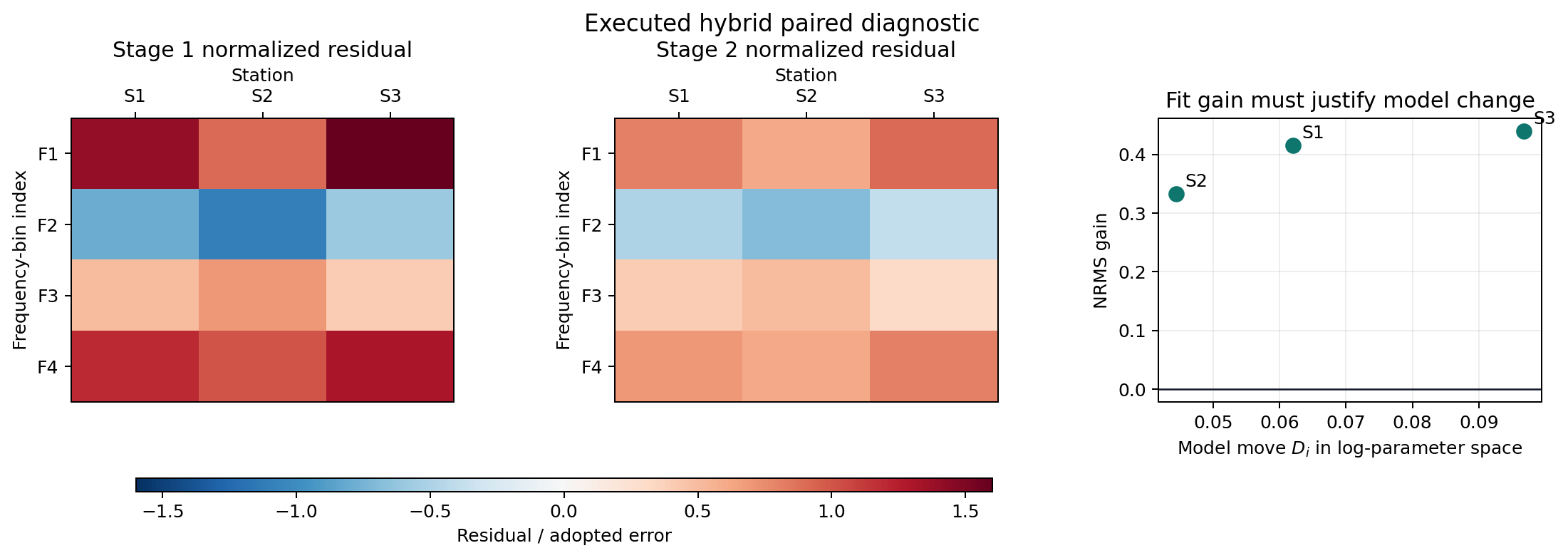
Executed paired diagnostic for the arrays above. The common residual color scale beneath the two heatmaps makes the contraction toward zero visible. Stations are columns labelled at the top and frequency bins run vertically. The final panel prevents that improvement from being separated from the model displacement defined by (11).#
All three stations move upward from the zero-gain line, so refinement improves the adopted response metric in every case. Station S3 moves farthest and also gains most; it deserves closer geological review than S2, whose similar gain is obtained with less model movement. This is the intended interpretation of the pair, not proof that any of these illustrative models is a WILLY subsurface result.
6.3.18.3. 1-D hybrid inversion#
pycsamt.ai.inversion.HybridInverter1D combines a fitted
pycsamt.ai.inversion.EMInverter1D with station-wise physics
refinement. The 1-D workflow is appropriate when each station can reasonably
be interpreted as a layered earth, or when the result is explicitly used as a
screening or initialization product before higher-dimensional inversion.
The repository does not ship checkpoints/amt1d_resnet.npz. The following
is therefore a reference run that becomes executable only after the
Training AI inversion models workflow has produced and validated that artifact. It must not
be quoted as an executed WILLY result from the documentation build.
>>> from pycsamt.ai.inversion import EMInverter1D, HybridInverter1D
>>>
>>> ai = EMInverter1D.load("checkpoints/amt1d_resnet.npz")
>>> hybrid = HybridInverter1D(
...     "data/AMT/WILLY_data/L18PLT",
...     ai_inverter=ai,
...     solver="mt1d",
...     comp="xy",
...     n_freqs=32,
...     max_iter=200,
...     smoothness_weight=0.005,
...     lr=5e-3,
... ).fit(verbose=True)
>>> models = hybrid.predict()
>>> stage1_models = hybrid.stage1_models()
>>> stage1_residuals = hybrid.residuals(stage=1)
>>> stage2_residuals = hybrid.residuals(stage=2)
The checkpoint or fitted object used for Stage 1 must be the exact artifact validated for the input representation. Record the checkpoint checksum, the frequency grid, component, transforms, and target parameterization. If the AI model predicts log-resistivity and log-thickness, the Stage-2 initialization inherits that representation before the physical solver converts it to positive parameters.
For each station, preserve:
the Stage-1 layered model;
the Stage-2 layered model;
residuals by frequency and component for both stages;
loss history and stopping iteration;
any stations where Stage 2 worsened response fit;
parameter floors, bounds, masks, and excluded frequencies.
The station-wise setting also makes failure localization clear. If only one station fails to improve, inspect that station before changing global weights: look for dead-band frequencies, missing phase, static-shifted apparent resistivity, component rotation, or a local dimensionality problem. If most stations fail to improve, the issue is more likely to be the AI starting model, the solver assumption, or the weighting of the Stage-2 objective.
There is a current solver-selection limitation worth making explicit:
solver="csamt1d" changes the public residual reconstruction to
CSAMT1DForward, but the differentiable
fit_station kernel receives no solver argument and always optimizes its MT
1-D recursion. Until those paths are unified, csamt1d is not evidence of a
CSAMT-specific Stage-2 objective. Treat such a run as experimental and verify
it with an independent CSAMT forward response; use solver="mt1d" for the
documented internally consistent path.
6.3.18.4. 2-D hybrid refinement#
pycsamt.ai.inversion.HybridInverter2D uses a fitted
pycsamt.ai.inversion.EMInverter2D to initialize a profile section and
then jointly refines all stations. The method is especially useful when a
U-Net-like section captures large-scale structure but needs explicit response
checking station by station.
EMInverter2D can be supplied as a fitted object
or as a saved checkpoint path; HybridInverter2D calls its inherited
load implementation for the latter. Retain the training configuration and
normalization state in either case–loading network weights does not by itself
reconstruct the scientific feature contract. The placeholder below uses the
fitted-object route so that dependency remains visible.
>>> from pycsamt.ai.inversion import HybridInverter2D
>>>
>>> # ai2d is a fitted EMInverter2D retained from training.
>>> hybrid = HybridInverter2D(
...     "data/AMT/WILLY_data/L18PLT",
...     ai_inverter=ai2d,
...     n_layers=10,
...     depth_max=2000.0,
...     n_freqs=32,
...     mode="te",
...     smoothness_weight=0.005,
...     lateral_weight=0.003,
...     epochs=150,
...     lr=5e-3,
... ).fit(verbose=True)
>>> stage1 = hybrid.stage1_section(as_log10=True)
>>> stage2 = hybrid.resistivity_section(as_log10=True)
>>> residuals_stage1 = hybrid.residuals(stage=1)
>>> residuals_stage2 = hybrid.residuals(stage=2)
The 2-D hybrid objective still depends on the solver assumptions used in the refinement step. If the implementation uses per-station 1-D response physics inside a laterally coupled section, say so directly in the report. Lateral smoothness can make neighbouring stations look geologically coherent, but it does not turn a pseudo-2-D response check into a full 2-D electromagnetic solver.
That is exactly what the current implementation does: every station is passed
through the differentiable layered 1-D MT recursion, while
\(\mathcal J_x\) couples adjacent station models. mode="te" selects
xy observations and mode="tm" selects yx. mode="both" does
not create two independent TE/TM residual blocks; it arithmetically averages
TE and TM apparent resistivity and phase before interpolation to the common
frequency grid. Use that mode only when this averaging is scientifically
defensible. For a genuine joint-mode or full 2-D response test, evaluate the
final model externally with the verified path in Solver-neutral Maxwell contracts.
Also note that residuals(stage=...) currently reports TE observations when
mode="both" because its diagnostic branch treats both like te;
those rows therefore do not reconstruct the averaged target optimized in
Stage 2. Compute the averaged-target residual explicitly or report separate
TE/TM external residuals rather than labelling that table as the training
objective.
Stage 1 may also be resampled along the station axis when the field profile has a different station count from the network’s fixed input shape. Missing panel values are filled by each channel/station frequency-column mean (or zero when the entire column is missing), the panel is linearly resized for the AI call, and the predicted section is resized back. Preserve both shapes and the missingness mask: interpolation can make an initializer visually smooth without adding observational support.
The controlled execution below isolates Stage 2 on seven synthetic stations.
The known response is generated independently with the public
MT1DForward; a deliberately biased warm start
is then refined for 140 Adam iterations by the same differentiable
fit_2d_joint kernel used by HybridInverter2D. The internal total
objective falls from above 1.3 to about 0.25, but the independently recomputed
response RMS changes from 0.549 to 0.575 and model RMSE from 0.377 to 0.638.
In other words, this run converges numerically while becoming less accurate
under two external checks.
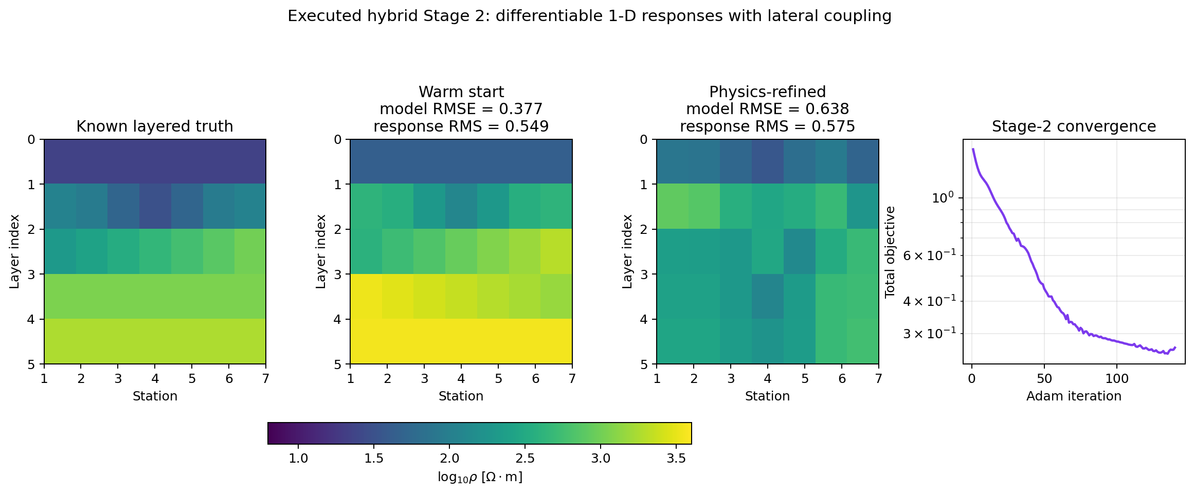
Executed pseudo-2-D refinement with a shared colour scale. Response RMS is recomputed with the public forward solver rather than read from the optimizer’s own loss history.#
The mismatch does not mean every hybrid run must worsen. It demonstrates that an internal differentiable recursion, its regularization, and an independent forward implementation are distinct numerical claims. A falling loss proves only that Adam is reducing the implemented objective. Require an external response reconstruction on the same frequencies and units before promoting Stage 2; where synthetic truth exists, retain model-space metrics as well. This diagnostic is especially important after either forward implementation changes.
The useful diagnostic is the difference between Stage 1 and Stage 2:
where \(z\) indexes depth and \(k\) indexes station or lateral position. Large coherent changes may indicate real correction, but they may also indicate that the supervised model was outside its training support. The response residuals decide whether the change improved the observation fit; the geology decides whether the changed structure is credible.
A 2-D hybrid report should show three aligned panels whenever possible: Stage-1 log-resistivity, Stage-2 log-resistivity, and \(\Delta\log_{10}\rho\). Put them on the same depth grid and color scale unless the purpose is explicitly to inspect a residual panel. The viewer should not have to infer improvement from different color limits. If several figures are needed, arrange them as a row or grid so the Stage-1 and Stage-2 relationship is visually immediate.
Depth parameterization matters. If Stage 1 predicts a section on one depth grid and Stage 2 optimizes another, document the interpolation. A sharp conductor can appear to move simply because the target grid changed. In decision-facing reports, quote interface depths or conductor-top depths from the final grid and preserve the Stage-1 grid in the reproducibility record.
6.3.18.5. 3-D and graph hybrid workflows#
pycsamt.ai.inversion.HybridInverter3D follows the same pattern with a
quasi-3-D, graph-based Stage-1 estimate. Its Stage-2 response term is assembled
from station-wise layered-earth responses and coupled by graph smoothness; it
is not a full 3-D Maxwell solver. The graph penalty should be tied to the
survey geometry, not chosen only because it makes a smoother volume. Record
the graph construction rule, edge radius, disconnected components, coordinate
system, and station exclusions. Stratify diagnostics by node degree and survey
edge position because graph models often look best in dense interior regions
and weakest near sparse boundaries.
This remains true when the Stage-1 GCN checkpoint was trained with
Genuine 3-D Maxwell training. Such training gives the initializer
experience of laterally coupled 3-D responses, but it does not change the
implemented Stage-2 operator. HybridInverter3D has no mt3d or
modem3d solver argument: pycsamt.ai.inversion._pinn_ops.fit_3d_joint()
evaluates a differentiable MT 1-D recursion independently at each station and
couples the model columns through the graph penalty. Consequently,
not one coupled residual \(\lVert F_{\mathrm{MT3D}}(\mathbf m)-\mathbf d^{\mathrm{obs}}\rVert\) over a shared conductivity volume. Equation (13) is therefore a quasi-3-D refinement even when Stage 1 came from genuine 3-D synthetic physics.
The returned resistivity_volume() has shape (layer, station). The word
volume describes graph-linked vertical columns; it is not a rectilinear
(z, y, x) output grid, and it should not be passed to a 3-D solver
without an explicit interpolation and support policy. Preserve station
coordinates, graph edges, per-station thicknesses, and any later gridding as
separate artifacts so display interpolation is not mistaken for recovered
3-D resolution.
A genuinely 3-D Stage 2 would need to map the Stage-1 model from its output
grid to a solver mesh, run MT3DAdapter or ModEm3DAdapter for
each candidate model, evaluate tensor residuals with observational errors,
and obtain derivatives through an adjoint, a differentiable 3-D operator, or
a documented derivative-free strategy. None of those optimization loops is
implemented by HybridInverter3D today. Calling the current result
ModEM-refined or 3-D Maxwell-refined would therefore be incorrect;
ModEM may be used afterward as an independent response audit, provided the
column-to-mesh mapping and backend provenance are recorded.
The current refinement also has no inactive-cell or terrain operator. Station elevations can influence plotted geometry or graph coordinates, but they do not place air cells into equation (13). A draped hybrid volume remains a visualization unless a terrain-capable 3-D forward problem is solved and validated separately.
The 2-D mode semantics carry into this path: mode="both" averages TE and
TM observables before optimization, and the built-in residual table does not
reconstruct that averaged target. Report separate externally recomputed TE and
TM residuals when both modes are part of the scientific claim.
When the field setting is not demonstrably 3-D, a 3-D hybrid result can still be useful as a consistency check. Report that narrower role. Do not promote a 3-D interpretation simply because the model class can output a volume.
For graph workflows, the Stage-1 prior can enter twice: once through the learned model and again through graph smoothness. That is not wrong, but it must be visible. A dense graph with a large \(\lambda_g\) can make a volume look stable even when the data support is sparse. Always compare graph hybrid output with a weaker graph or identity-graph ablation before claiming that the volume is physically resolved.
6.3.18.6. Agent-assisted hybrid runs#
pycsamt.agents.HybridInversionAgent wraps the 1-D, 2-D, and 3-D
classes and returns a standardized result package with residual tables,
figures, and Stage-1 versus Stage-2 summaries.
>>> from pycsamt.agents import HybridInversionAgent
>>> from pycsamt.ai.inversion import EMInverter1D
>>>
>>> ai = EMInverter1D.load("checkpoints/amt1d_resnet.npz")
>>> agent = HybridInversionAgent(
...     dim=1,
...     max_iter=100,
...     smoothness_weight=0.005,
...     lr=5e-3,
...     api_key="",
... )
>>> result = agent.execute({
...     "path": "data/AMT/WILLY_data/L18PLT",
...     "ai_inverter": ai,
...     "output_dir": "outputs/hybrid/L18_1d",
... })
>>> result.status
'success'
>>> sorted(result.data)[:5]
['convergence_df', 'figure_paths', 'figures', 'inverter', 'models']
Use the agent when standardized packaging is more important than exposing every low-level constructor option. Use the inverter classes directly when component choice, mode, depth grid, graph geometry, or persistence behavior must be controlled exactly.
At the current API boundary, use the agent’s executed path for 1-D only. Its
2-D and 3-D private dispatch still forwards legacy solver/max_iter
arguments and requests legacy stage-selecting output signatures that the
current HybridInverter2D and HybridInverter3D constructors
do not accept. Those dimensions should be run through the inverter classes
directly until the convenience wrapper is updated and integration-tested.
An agent returning failed is not a scientific Stage-2 result.
The agent result should be treated as a convenience layer, not as the only scientific record. Keep the underlying fitted inverter when the analysis may need later residual recomputation, alternative plotting, or sensitivity tests. If the agent saves figure paths, make sure the output directory also contains the parameters that generated those figures; a plot without its weights and mask is not reproducible evidence.
6.3.18.7. Convergence and stopping#
Hybrid optimization starts from a meaningful model, so the loss curve often falls quickly and then flattens. Stopping should not be based only on the last loss value. Inspect:
whether data misfit and regularization terms move in the same direction;
whether Stage 2 improves RMS misfit relative to Stage 1;
whether the model keeps changing after response improvement has saturated;
whether a few stations dominate the remaining loss;
whether different seeds or small perturbations of Stage 1 converge to the same interpretation.
When only the total loss is available, compare early, selected, and final iterations rather than reporting the final model automatically. A later iteration can have slightly lower loss but a less interpretable section if the decrease comes from a narrow noisy band. For reproducibility, record the selected epoch or iteration and the reason it was selected.
6.3.18.8. Sensitivity design#
A hybrid run should be accompanied by a small sensitivity set. The goal is not to produce a gallery of alternatives; it is to test whether the scientific claim depends on one fragile setting. Useful perturbations are:
Stage-1 checkpoint from a different seed or architecture;
\(\lambda_z\), \(\lambda_x\), or \(\lambda_g\) multiplied and divided by a small factor;
TE, TM, or both modes where the data support allows it;
removal of suspect frequencies or stations;
mild perturbation of the Stage-1 model before refinement;
alternative error floors for apparent resistivity and phase;
a classical inversion or PINN run started from a neutral model.
The scientific result is stronger when the target conductor, interface, or resistive body remains in the same approximate place across acceptable scenarios. It is weaker when only one setting produces the desired structure.
6.3.18.9. What to compare#
Hybrid validation is a paired comparison. Every case has at least two predictions from the same input: the AI Stage-1 estimate and the physics-refined Stage-2 estimate. Compare them on identical masks and units:
Stage-1 and Stage-2 response-space metric values;
Stage-1 and Stage-2 model-space metric values where synthetic or withheld truth exists;
residual trends by frequency, station, and component;
model change in log-resistivity, thickness, and interface depth;
improvement over the agreed baseline model;
sensitivity to regularization weights, learning rate, and iteration count;
convergence from different seeds or perturbed Stage-1 starts;
field consistency with independent geology, wells, or classical inversion.
The expected outcome is not always “Stage 2 changes the model.” A small model change with a clear residual improvement can be excellent. A large model change with little response improvement is a warning that the optimizer may be using regularization freedom or data noise rather than recovering structure.
A simple decision matrix helps keep this interpretation consistent:
Observation |
Likely reading |
Action |
|---|---|---|
Stage 2 improves response fit and makes a small model move. |
The AI estimate was close and physics refinement corrected it. |
Accept if validation gates and field evidence also pass. |
Stage 2 improves response fit but makes a large model move. |
The AI estimate may be outside local support, or the data require structure absent from Stage 1. |
Treat as conditional; run sensitivity and independent checks. |
Stage 2 changes the model but response fit barely improves. |
The refinement is probably weakly constrained. |
Do not promote without stronger evidence. |
Stage 2 worsens response fit. |
The objective, weights, masks, or starting model may be incompatible. |
Inspect residuals and revert to Stage 1 or redesign the run. |
Stage 2 improves global fit but worsens critical stations. |
A mean score is hiding local failure. |
Report station-level limitations or narrow the operating envelope. |
6.3.18.10. Reporting requirements#
A hybrid report should make the transition from AI estimate to physics refinement reproducible:
Stage-1 checkpoint identity, checksum, training domain, and feature contract;
observed data source, component, frequency grid, masks, and units;
solver, dimensionality, parameterization, bounds, and floors;
objective weights \(\lambda_z\), \(\lambda_x\), and \(\lambda_g\);
optimizer, learning rate, iteration count, stopping rule, and device;
Stage-1 and Stage-2 sections or models shown together;
Stage-1 and Stage-2 residual tables and figures;
response reconstruction settings and residual definition;
uncertainty or scenario ensemble results when the interpretation depends on the refined model;
final status: accepted, conditional, or rejected for the declared use.
For reproducibility, store the raw Stage-1 output before any positivity floor or solver-specific conversion. Floors are sometimes necessary to keep the physics step stable, but they can also hide an invalid AI prediction. The reader should be able to see whether Stage 2 refined a credible starting model or corrected a starting model that was already outside the allowed range.
6.3.18.11. Common failure modes#
Hybrid inversion can fail quietly. Watch for:
Stage 2 improves the total scalar loss but worsens a critical frequency band;
the final model is nearly identical to Stage 1 because the optimizer stalled;
response fit improves only after excessive smoothing removes target structure;
a strong domain gap is treated as a refinement problem;
lateral or graph regularization creates coherence unsupported by the data;
genuine 3-D Stage-1 training is reported as if Stage 2 also solved coupled 3-D Maxwell physics;
a gridded or terrain-draped
(layer, station)result is described as a solver-native 3-D volume;the Stage-1 checkpoint is restored without its preprocessing normalizers;
synthetic validation shows improvement, but field residuals remain systematic;
only the final section is reported, hiding Stage-1 dependence.
The safest conclusion is often conditional: the hybrid result is accepted inside a declared operating envelope, with classical review or independent evidence required where the Stage-2 correction is large.
6.3.18.12. Next steps#
Use Physics-informed 2-D inversion when the workflow starts directly from physics-informed optimization rather than from a supervised AI estimate. Use AI inversion validation to decide whether Stage 2 truly improves the model, and use AI inversion reporting to package both stages as auditable evidence.