6.3.2. Architecture roadmap#

The pages under AI inversion concepts, AI inversion data preparation, AI model selection, Training AI inversion models, AI inversion inference, AI inversion validation, AI inversion uncertainty, Hybrid AI and physics inversion, Physics-informed 2-D inversion, AI inversion agents, and AI inversion reporting document the Inv2DAgent/ Inv3DAgent workflow that predates this roadmap. Both agents started as smoke/demo implementations: they inverted each station independently against station-wise 1-D (em1d) synthetic physics, then tiled the per-station results into a pseudo-2-D or pseudo-3-D section. Because each station was solved in isolation, nothing enforced lateral continuity between neighbours, so a raw, native-cell rendering of that tiling looked patchy rather than smooth. That physics="mt1d" path still exists, unconditionally, as Inv2DAgent’s default — but it is no longer the only path. An opt-in physics="mt2d" mode now generates genuinely 2-D correlated training models and solves them with a verified 2-D Maxwell backend before training a U-Net on the result, described below in Wired into the agents. Inv3DAgent has not made the same transition yet: it still shares layered station parameters through a spatial graph rather than solving a 3-D forward problem.

Do not mistake smoothness for resolution

A published figure that looks smooth may simply be display interpolation, unrelated to whether the underlying cells were actually resolved. Genuine smoothness in a released model should come from a network resolving spatially correlated structure, learned through the loss terms in Loss functions for scientific inversion, not from a post-hoc rendering choice. Save and label both the native-cell and the interpolated version of a section, and publish it alongside response residuals, uncertainty, and a comparison with an established classical inversion — never display interpolation alone as evidence of recovered resolution.

This is the reason a lower-level architecture has been built underneath the existing agents rather than only tuning the agents themselves. A single U-Net trained on tiled, independent 1-D columns cannot be described as genuine 2-D or 3-D electromagnetic inversion, regardless of how its output is rendered — it has to consume real 2-D/3-D forward physics, spatially correlated training models, a staged loss with explicit spatial regularization and response fit, and validated recovery/uncertainty evidence, in that order. The package map below is that architecture; the sections after it report, honestly, how much of it is verified today rather than only planned.

Roadmap language is deliberately cumulative. Implemented means that a public API exists. Verified adds focused tests or physical benchmarks. Wired means that an agent or dataset workflow actually consumes the API. Gated adds a predeclared, automatically evaluated acceptance criterion, and released adds a blind field evaluation with archived artifacts. Thus, an implemented solver is not automatically a verified solver, and a verified loss function is not automatically part of an accepted inversion workflow. For milestone \(m\), the release condition can be written compactly as

(1)#\[R_m = I_m \land V_m \land W_m \land G_m \land B_m,\]

where \(I_m\), \(V_m\), \(W_m\), \(G_m\), and \(B_m\) denote implementation, verification, workflow wiring, automatic gate, and blind-evaluation evidence. Equation (1) is a logical contract, not a numerical score: one missing condition prevents a release claim even when the other four are satisfied.

6.3.2.1. Package map#

Each row below is one building block of the architecture. All of them are usable as libraries today; Wired into the agents covers which ones are actually consumed end-to-end by an agent, as opposed to only unit-tested in isolation.

Package	Role	Guide page
`pycsamt.ai.data`	Canonical impedance tensors, masks, normalization state, and dataset manifests shared by every later stage.	Canonical data contracts
`pycsamt.ai.geology`	Correlated random fields, layered geology, faults/lenses, and topography for synthetic training models.	Correlated geological priors
`pycsamt.ai.domain_gap`	Heteroscedastic noise, error floors, static shift, galvanic distortion, dropout, outliers, and coordinate perturbations, with parameter ranges that can be fitted directly from a real survey’s own QC diagnostics rather than guessed.	Domain-gap and noise simulation
`pycsamt.forward.maxwell`	Solver-neutral 2-D/3-D Maxwell problem/result contracts, a backend registry, and concrete adapters for a verified 2-D solver, a research-only 3-D solver, and an external ModEM adapter.	Solver-neutral Maxwell contracts
`pycsamt.ai.training.dataset2d`	Wires `geology` fields through a `maxwell` backend, batched and cached, into versioned `SurveyData` training pairs.	2-D Maxwell training-data generation
`pycsamt.ai.training.dataset3d`	Wires `geology` volumes through `MT3DAdapter` on a padded, non-uniform mesh, into the same versioned `SurveyData` training-pair shape as the 2-D generator. M8’s research slice, not yet its production backend (see M8 above).	3-D Maxwell training-data generation
`pycsamt.ai.losses`	The staged training objective: data fit, spatial regularization, response consistency, boundary constraints, and uncertainty terms.	Loss functions for scientific inversion
`pycsamt.ai.validation`	Synthetic-recovery diagnostics, response-residual reports, calibration curves, and out-of-distribution checks.	Recovery, residual, and OOD diagnostics
`pycsamt.ai.experiments`	Immutable experiment configuration, seed lineage, and acceptance-gate evaluation for reproducible runs.	Reproducible experiment configuration

6.3.2.2. The 3-D Maxwell equation and the production-backend choice#

The equation maxwell targets for a 3-D problem, with one documented time convention fixed per problem (MaxwellProblem accepts either exp(+iwt) or exp(-iwt), never both silently), is

(2)#\[\nabla\times\left(\mu^{-1}\nabla\times\mathbf E\right) + i\omega\sigma\mathbf E = \mathbf s,\]

with complex electric field \(\mathbf E\), angular frequency \(\omega\), permeability \(\mu\), conductivity \(\sigma\) (anisotropic where a backend declares that support), and source term \(\mathbf s\). Equation (2) is the same one Solver-neutral Maxwell contracts’s 2-D adapter already solves on a reduced TE/TM formulation. Extending it to a genuine 3-D solve raises a practical question: solve it directly in-house, or route it through a trusted external backend, the way Occam2D and MARE2DEM already do for other methods in this package.

A direct sparse solve does not scale to production 3-D EM. Timing a direct factorization against an unpreconditioned iterative solve at increasing problem size shows direct-solve cost growing close to quadratically with cell count, which extrapolates to tens of minutes per single frequency/polarization solve at a realistic 3-D mesh size — before multiplying by polarizations, frequencies, and the hundreds to thousands of realizations a training dataset needs. No verified Python 3-D EM package (SimPEG, discretize, emg3d, pygimli) is installed in this environment, and the existing MT3DForward is explicitly Quasi-3-D: it averages two independent 2-D cross-section solves rather than solving equation (2) directly, so it is not a genuine 3-D candidate either. Production 3-D work therefore targets a verified external backend; an in-house solver is kept research-only until it can be paired with a problem-specific preconditioner, itself a substantial and distinct numerical effort.

Two adapters exist as a direct consequence:

ModEm3DAdapter: Wraps the vendored ModEM Fortran solver (pycsamt/models/modem/_source) as a BaseExternalMaxwellAdapter subclass, reusing ModEM’s own file I/O rather than a second parser. This is the intended production adapter. No compiled Mod3DMT binary is committed to the repository (it is a local build artifact — see pycsamt/models/modem/_source/README for build instructions), but one has been built and used to validate this adapter against both analytic benchmarks with real margin, so its verified_benchmarks reports ("half-space", "layered-earth"). That validation surfaced and fixed five real bugs spanning the vendored Makefile, this adapter’s own command-building and the shared external-executable resolver, the WS-format model reader/writer, and a genuine out-of-bounds read in ModEM’s own air-layer setup for grids with fewer than 10 earth z-cells (now an explicit preflight rejection) — see the module docstring and the M6 ADR’s 2026-07-29 update for the full account.
MT3DAdapter: A genuine, in-house discrete curl-curl solver on a Cartesian Yee grid (cell widths may be non-uniform per axis, e.g. a padded mesh), provided as an explicit research-only alternative and capped at 6,000 cells by its own declared capabilities. On a padded, non-uniform calibrated mesh it passes both the analytic half-space and layered-earth benchmarks, so its verified_benchmarks reports ("half-space", "layered-earth"). Small-grid/research-only status is unrelated to this and still applies: it exists because a direct sparse solve does not scale to realistic production 3-D mesh sizes (see the M6 architecture-decision record), not because of any remaining accuracy gap.

6.3.2.3. What is verified today#

None of the claims above are worth much without a way to check them against the running code, so check the registry directly instead of trusting this page’s prose:

>>> from pycsamt.forward.maxwell import (
...     register_mt2d_backend,
...     register_modem3d_backend,
...     list_backends,
... )
>>> register_mt2d_backend()
>>> register_modem3d_backend()
>>> for name, info in sorted(list_backends().items()):
...     cap = info["capabilities"]
...     print(
...         name, "dims=", cap["dimensions"],
...         "verified=", cap["verified_benchmarks"],
...         "available=", info["available"],
...     )
modem3d dims= [3] verified= [] available= False
mt2d dims= [2] verified= ['half-space', 'layered-earth'] available= True

mt2d reports two verified benchmarks and is available in any environment, since it wraps in-repo Python physics. modem3d reports zero verified benchmarks and available=False here, because resolve_executable() cannot find a compiled ModEM binary — this is exactly the honesty the verified_benchmarks field exists to enforce: a backend’s benchmark status is read from its registration, not asserted in documentation. MT3DAdapter does not appear at all, because it has no register_mt3d_backend entry point; being research-only and cell-capped, it is meant to be constructed directly, not routed to through the registry a production dataset generator would use.

6.3.2.4. Wired into the agents#

A library existing under pycsamt.ai or pycsamt.forward.maxwell does not by itself change what Inv2DAgent or Inv3DAgent do. Inv2DAgent now exposes a physics argument that chooses between the two:

physics="mt1d" (default): Unchanged from the original smoke/demo path: independent 1-D forward models tiled into a profile-shaped array. Kept as the default and as an explicit fallback, so a known baseline is always available to compare against.
physics="mt2d" (opt-in): Generates spatially correlated 2-D training models with geology, solves them with the verified MT2DAdapter through generate_2d_maxwell_dataset(), and can add the spatial-regularization terms from Loss functions for scientific inversion (lambda_x, lambda_z, lambda_tv) to fit(). Only the TE-mode (zxy) response is used for training here, even though 2-D Maxwell training-data generation now validates the TM-mode (zyx) response too — this agent’s feature layout is still TE-only, so it does not ask for the extra, currently-unused mode. Where a held-out synthetic split exists, a genuine synthetic recovery check against known-truth resistivity is attached to the result through recovery_report() — the one place in this workflow where “recovery” evidence is actually available, since field surveys carry no ground truth to compare against.

This is real wiring, not a description of intent: both physics modes run end-to-end against bundled EDI data in the agent’s own test suite. It is also an incomplete one. The mt2d path currently places stations on a synthetic uniform grid rather than the field survey’s actual geometry, no automated evaluation of the M5 acceptance threshold exists yet (only the recovery check above, which is necessary but not sufficient), and the spatial-regularization terms train only on the PyTorch backend — selecting them under TensorFlow raises rather than silently falling back to an unregularized fit. Inv3DAgent has not been touched by any of this: it remains a Quasi-3-D-adjacent graph model over per-station layered parameters, sharing information through station adjacency rather than solving equation (2) in three dimensions, and Solver-neutral Maxwell contracts’s two 3-D adapters are not yet its data source.

6.3.2.5. Milestone status#

The architecture is organized into eleven development stages, M0 through M10, each gated by an explicit acceptance criterion before it can be called complete. The table below reports where each stage genuinely stands today.

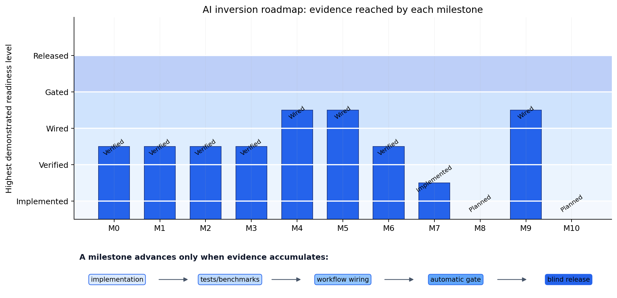
Readiness level reached by AI inversion milestones M0 through M10 — The highest demonstrated readiness level for each milestone. Bars stop at the available evidence; they do not estimate percentage completion.#

The concentration of blue bars at verified and wired is informative. The reusable 2-D components are no longer merely proposals, but automatic acceptance and blind release remain the bottleneck. M7 is different: its production adapter is implemented, yet verification cannot advance until a compiled ModEM executable is available. M8 and M10 are shown as planned, so their zero-height bars must not be read as failed experiments.

Milestone	Scope	Status
M0	Baseline freeze and reproducibility	Verified. Experiment configuration and seed/split manifests exist and have focused tests; see Reproducible experiment configuration. They support later gates, but do not themselves constitute a field release.
M1	Survey data contract and WILLY audit	Verified. `SurveyData` is exercised on WILLY in Canonical data contracts; frequency coverage, dimensionality, and static-shift/domain-fit evidence are reported across Canonical data contracts, AI model selection, and Domain-gap and noise simulation. These checks are documented and reproducible, although they are not yet exported as one signed release artifact.
M2	Correlated geological priors	Verified as a library. Correlated geological priors exercises correlated fields, layers, faults, lenses, topographic surfaces, and 3-D composition with reproducible diagnostic figures. Ensemble ranges still need to be frozen for each survey-specific experiment rather than treated as universal geological assumptions.
M3	Domain-gap and noise simulator	Verified. `pycsamt.ai.domain_gap` fits noise, dropout, and distortion ranges from real WILLY QC diagnostics and is tested against that survey, not only against synthetic self-tests.
M4	Genuine 2-D electromagnetic forward path	Wired. `MT2DAdapter` passes both analytic benchmarks; contracts, mesh, cache, batching, and the external-adapter base are tested, and 2-D Maxwell training-data generation consumes the backend to generate training pairs (Solver-neutral Maxwell contracts).
M5	Response-aware 2-D learning	Wired, not gated. The staged loss and validation libraries exist; `Inv2DAgent(physics="mt2d")` wires them together end-to-end (Wired into the agents); the gate’s own held-out normalized-RMS threshold is not yet evaluated automatically.
M6	3-D Maxwell solver feasibility and specification	Decided. Production 3-D work targets an external ModEM backend; an in-house production solver is not pursued — see What is verified today above.
M7	Verified 3-D forward backend	Substantively addressed for the ModEM path. `ModEm3DAdapter` was validated against both analytic limits using a real compiled `Mod3DMT` (a local build artifact, not committed — see `pycsamt/models/modem/_source/README`), which surfaced and fixed five real bugs (a vendored Makefile gap, a `resolve_executable` PATHEXT gap, a missing ModEM CLI argument, a WS-format header mismatch, and a genuine out-of-bounds read in ModEM’s own air-layer sizing for grids with fewer than 10 earth z-cells). Remaining open items: ModEM license terms are still unconfirmed with the OSU authors, and only the two analytic limits (not the 2-D extrusion, isolated 3-D body, non-uniform mesh, or MPI-build cases) have been checked. `MT3DAdapter` is a research-only exception, verified at both the half-space and layered-earth limits (not a production backend regardless — see M6).
M8	Correlated 3-D training and spatial model	Not started against the verified ModEM backend; a research slice exists but is explicitly not this milestone’s production backend — `Inv3DAgent(physics="mt3d")` trains on genuinely 3-D volumes solved with `MT3DAdapter` (via 3-D Maxwell training-data generation), not `ModEm3DAdapter`.
M9	Hybrid inversion and uncertainty, on this architecture	Wired on the earlier architecture. The 1-D, 2-D, and 3-D hybrid classes perform staged AI initialization and physics refinement, and Hybrid AI and physics inversion documents their outputs and uncertainty checks. They do not yet consume the complete `pycsamt.ai.losses`, `pycsamt.ai.validation`, and `pycsamt.ai.experiments` acceptance stack, so M9 is not gated or release-ready.
M10	WILLY blind evaluation and release	Not started; depends on M5 through M9.

Read this table with the linked package pages and the running APIs. Those pages describe limitations beside the affected operation, where they are less likely to be separated from the example than in a generic status box. If a future implementation changes before this summary does, the executable examples, backend capability declarations, and tests are the authoritative evidence.

6.3.2.6. Next steps#

Continue with the package-level pages, each covering one row of the map above with a runnable example:

For the complete Inv2DAgent/Inv3DAgent workflow built on top of these packages, continue with AI inversion data preparation, AI model selection, Training AI inversion models, AI inversion inference, AI inversion validation, AI inversion uncertainty, Hybrid AI and physics inversion, Physics-informed 2-D inversion, AI inversion agents, and AI inversion reporting.