6.3.10. Recovery, residual, and OOD diagnostics#

Loss functions for scientific inversion shapes what a network is trained to minimize; pycsamt.ai.validation is where the result gets checked afterwards, by someone other than the optimizer. It splits that checking into four independent areas rather than one aggregate score: a model-space metric for known-truth synthetic recovery (recovery), a response-space metric broken down by where it comes from (residuals), whether a declared predictive uncertainty deserves trust (calibration), and an out-of-distribution diagnostic for inputs the training support never covered (ood). Plotting stays in pycsamt.ai.plot; every number a validation figure draws comes from here. The older, still-active AI inversion validation page documents Inv2DAgent/Inv3DAgent’s own separate, built-in validation protocol; this package is the newer, modular library described in Architecture roadmap, and — as the closing section below shows — the two are already partly connected rather than entirely separate.

The public API is small enough to map explicitly. Report classes are frozen dataclasses: their numerical arrays are read-only, which prevents a plotting step from silently changing evidence after it has been computed.

Validation API and the question each object answers#
Area	Functions	Returned evidence
Known-truth recovery	`recovery_report()`, `structural_similarity()`, `depth_profile_rmse()`, and `depth_profile_mae()`	`RecoveryReport` combines global error, \(R^2\), SSIM, valid-cell count, and depth profiles.
Forward-response fit	`response_residual_report()` and `response_residual_report_from_contracts()`	`ResponseResidualReport` retains overall, station, frequency, and component reductions with axis labels.
Predictive uncertainty	`reliability_curve()`, `empirical_coverage()`, and `predictive_sharpness()`	`ReliabilityCurve` keeps nominal levels, observed coverage, calibration loss, sharpness, and sample count.
Training-support screening	`ood_score()` and `flag_out_of_distribution()`	`OODReport` keeps scores, threshold, flags, method, reference size, feature count, and flagged fraction.

These outputs are complementary. Recovery asks whether a known synthetic earth was reconstructed; response residuals ask whether its forward response fits observations; calibration asks whether stated intervals attain their coverage; OOD screening asks whether applying the predictor was supported in the first place. None is a surrogate for another.

6.3.10.1. Scoring recovery when the truth is known#

A field survey has no ground truth to compare against, but a synthetic realization from generate_2d_maxwell_dataset() does, which is exactly what makes recovery_report() possible: masked RMSE and MAE reusing model’s own reductions, an \(R^2\) against the true section’s own variance, a windowed structural similarity index, and a per-depth breakdown. Standing in for a trained network’s prediction with one of this package’s own realizations, lightly perturbed and made deliberately worse at the bottom row:

For valid model cells \(\mathcal V\), prediction \(\hat m_i\), and known truth \(m_i\), the three scalar recovery summaries are

(1)#\[\begin{split}\begin{aligned} \operatorname{RMSE}_m &= \sqrt{\frac{1}{|\mathcal V|} \sum_{i\in\mathcal V}(\hat m_i-m_i)^2},\\ \operatorname{MAE}_m &= \frac{1}{|\mathcal V|} \sum_{i\in\mathcal V}|\hat m_i-m_i|,\\ R^2_m &= 1-\frac{\sum_{i\in\mathcal V}(m_i-\hat m_i)^2} {\sum_{i\in\mathcal V}(m_i-\bar m)^2}. \end{aligned}\end{split}\]

Use one model parameterization consistently on both sides. In the example that parameter is \(m=\log_{10}\rho\), so an RMSE of 0.1 means error in log-resistivity, not 0.1 \(\Omega\,\mathrm m\). A factor-of-ten resistivity error corresponds to one log unit. The valid mask combines the explicit valid argument with finite cells in both arrays; a depth row with no valid cell is retained as nan rather than being reported as zero.

>>> import numpy as np
>>> from pycsamt.ai.geology import GeologyGrid
>>> from pycsamt.ai.training.dataset2d import (
...     Maxwell2DDatasetConfig, generate_2d_maxwell_dataset,
... )
>>> from pycsamt.ai.validation import recovery_report

>>> grid = GeologyGrid.regular_2d(nx=10, nz=8, dx_m=300, dz_m=150)
>>> config = Maxwell2DDatasetConfig(
...     dataset_id="sv-demo", grid=grid,
...     correlation_length_x_m=(600.0, 1200.0),
...     correlation_length_z_m=(200.0, 400.0),
...     frequencies_hz=np.logspace(0, 4, 12),
...     station_x_m=list(np.linspace(500.0, 2500.0, 10)),
...     n_realizations=6, seed=7,
...     log_resistivity_mean=2.0, log_resistivity_std=0.4,
...     validation_fraction=0.0, test_fraction=0.0,
... )
>>> dataset = generate_2d_maxwell_dataset(config)
>>> true_log_rho = np.log10(dataset.samples[0].resistivity_ohm_m)

>>> rng = np.random.default_rng(11)
>>> pred_log_rho = true_log_rho + rng.normal(scale=0.08, size=true_log_rho.shape)
>>> pred_log_rho[-1, :] += 0.35  # a network that degrades at depth

>>> report = recovery_report(pred_log_rho, true_log_rho, compute_ssim=True, ssim_window=3)
>>> round(report.rmse, 4), round(report.mae, 4), round(report.r2, 4)
(0.1533, 0.0971, 0.8531)
>>> round(report.ssim, 4)
0.8553
>>> np.round(report.depth_rmse, 4)
array([0.0728, 0.0538, 0.0872, 0.0522, 0.0717, 0.0793, 0.0411, 0.3954])

The global RMSE alone (0.153) hides exactly what report.depth_rmse shows plainly: seven of eight layers sit near 0.05-0.09, and the bottom layer alone is at 0.395 — the injected depth-dependent bias would be invisible in one aggregate number. structural_similarity(), used inside report.ssim above, follows the windowed luminance/contrast/structure formulation of Wang et al. (2004),

(2)#\[\mathrm{SSIM}(x, y) = \frac{(2\mu_x\mu_y + c_1)(2\sigma_{xy} + c_2)} {(\mu_x^2 + \mu_y^2 + c_1)(\sigma_x^2 + \sigma_y^2 + c_2)},\]

with \(\mu\), \(\sigma^2\), and \(\sigma_{xy}\) the windowed mean, variance, and covariance and \(c_1\), \(c_2\) small stabilizing constants proportional to the data range — it has no defined masking rule, so it is skipped (ssim=None in RecoveryReport) whenever the grid is partially masked or smaller than the requested window, rather than silently computed over an incomplete comparison. depth_profile_rmse() and depth_profile_mae() are also available standalone, for a report that only needs the per-layer breakdown without the rest.

6.3.10.2. Breaking a response residual down by where it comes from#

Recovery only applies where a true model exists. residuals instead breaks response’s complex-impedance residual down by station, frequency, and component — the diagnostic that still works on a field survey with no synthetic truth at all, since it compares a forward-simulated response against an observed one rather than a predicted model against a true one. A residual that is large everywhere means something different from one localized to a handful of stations, and only the second shape is visible once it is broken down:

>>> from pycsamt.ai.validation import response_residual_report

>>> rng = np.random.default_rng(5)
>>> n_sta, n_freq, n_comp = 4, 3, 2
>>> z_true = (
...     rng.normal(scale=40, size=(n_sta, n_freq, n_comp))
...     + 1j * rng.normal(scale=40, size=(n_sta, n_freq, n_comp))
...     + (60 + 40j)
... )
>>> z_pred = z_true.copy()
>>> z_pred[2:, :, 1] += (15 + 10j)  # bias only zyx at stations S3/S4

>>> report = response_residual_report(
...     z_pred, z_true, kind="l2",
...     station_names=["S1", "S2", "S3", "S4"],
...     frequencies_hz=[1.0, 10.0, 100.0],
...     components=["zxy", "zyx"],
... )
>>> report.overall.value
81.25000000000001
>>> np.round(report.by_station, 3)
array([  0. ,   0. , 162.5, 162.5])
>>> np.round(report.by_frequency, 3)
array([81.25, 81.25, 81.25])
>>> np.round(report.by_component, 3)
array([  0. , 162.5])

The overall value of 81.25 gives no hint that the true residual is zero at two of four stations; by_station and by_component localize it exactly to S3/S4 and zyx, while by_frequency stays flat because the injected bias does not depend on frequency — three different projections of the same underlying array, each answering a different question about the same misfit. response_residual_report_from_contracts() skips the manual array handling the same way response_loss_from_contracts() does (see Loss functions for scientific inversion), taking a ForwardResult and a SurveyData directly and refusing to run on station, component, or frequency sets that are not identically ordered.

With observed standard error \(s_{sfc}\) at station \(s\), frequency \(f\), and component \(c\), the kind="l2" cell penalty and its global reduction are

(3)#\[q_{sfc} = \left|\frac{\hat Z_{sfc}-Z_{sfc}}{s_{sfc}}\right|^2, \qquad \bar q = \frac{\sum_{sfc}v_{sfc}q_{sfc}} {\sum_{sfc}v_{sfc}},\]

where \(v_{sfc}\) is the combined finite-data and validity mask. The reported overall.value is \(\bar q\), a mean squared normalized residual, not its square root. When errors=None, the division by \(s_{sfc}\) is omitted and the result carries squared impedance units; such an unnormalized value should not be compared between surveys with different impedance scales. Axis summaries apply the same masked mean while retaining one axis, so an empty station or frequency becomes nan.

6.3.10.3. Checking whether declared uncertainty deserves trust#

A network’s declared confidence is only useful if it is honest. reliability_curve() checks that directly: at each of several nominal confidence levels, what fraction of a held-out calibration set’s true values actually fall inside the predicted mean +/- z(level) * std interval — the same Gaussian parameterization gaussian_nll_loss() trains against, so a network trained with that loss can be checked with the metric that matches it. Two models with identical predicted means but different declared standard deviations make the point concrete: one whose declared spread matches the data’s real scatter, and one that is simply overconfident:

>>> from pycsamt.ai.validation import reliability_curve

>>> rng = np.random.default_rng(21)
>>> true = rng.normal(loc=0.0, scale=1.0, size=2000)
>>> mean = np.zeros(2000)

>>> curve_ok = reliability_curve(true, mean, np.ones(2000), levels=[0.5, 0.8, 0.9, 0.95])
>>> np.round(curve_ok.coverage, 3)
array([0.514, 0.821, 0.908, 0.961])
>>> round(curve_ok.calibration.value, 5), curve_ok.sharpness
(0.0002, 1.0)

>>> curve_bad = reliability_curve(true, mean, np.full(2000, 0.5), levels=[0.5, 0.8, 0.9, 0.95])
>>> np.round(curve_bad.coverage, 3)
array([0.27 , 0.496, 0.606, 0.681])
>>> round(curve_bad.calibration.value, 5), curve_bad.sharpness
(0.07603, 0.5)

Sharpness alone would call the second model better: a declared standard deviation of 0.5 is a tighter, more confident interval than 1.0. Its coverage tells the opposite story — a nominal 90% interval only actually contains the true value 61% of the time, because the declared spread understates the data’s real scatter by exactly the factor it was shrunk by. predictive_sharpness() is therefore documented, and should be read, as meaningful only alongside good calibration, never as a quality signal by itself.

For a two-sided Gaussian interval at nominal level \(\alpha\), empirical coverage and the default squared calibration penalty are

(4)#\[\widehat C(\alpha) = \frac{1}{N}\sum_{i=1}^{N} \mathbb 1\!\left[ |m_i-\hat\mu_i| \leq \Phi^{-1}\!\left(\frac{1+\alpha}{2}\right)\hat\sigma_i \right], \qquad L_{\mathrm{cal}} = \frac{1}{K}\sum_{k=1}^{K} \left[\widehat C(\alpha_k)-\alpha_k\right]^2.\]

Here \(\Phi^{-1}\) is the standard-normal quantile and \(K\) is the number of requested levels. Equation (4) explains why one 90% coverage number is insufficient: a model can happen to cross the ideal line once while being systematically miscalibrated elsewhere. The full curve exposes that shape. It also explains why this check belongs on held-out truth—using training targets would measure confidence on data already used to fit the predictor.

6.3.10.4. Flagging predictions the training distribution never covered#

None of the checks above say anything about an input a network was never trained near in the first place. ood_score() measures that directly against a reference set of training feature vectors, either by Mahalanobis distance from the reference mean and covariance,

(5)#\[d(\mathbf x) = \sqrt{(\mathbf x - \boldsymbol\mu)^{\!\top} \boldsymbol\Sigma^{-1} (\mathbf x - \boldsymbol\mu)},\]

which assumes an elliptical reference distribution and needs more reference samples than features to invert \(\boldsymbol\Sigma\), or by plain Euclidean distance to the \(k\)-th nearest reference point, which makes no distributional assumption at all. flag_out_of_distribution() turns either score into a flag by comparing against a quantile of the reference set’s own leave-one-out self-scores — “how unusual is a typical reference point” — rather than an arbitrary fixed number. Using each realization’s own depth- and lateral-roughness (the standard deviation of its first difference along each axis) as a two-feature summary of geological character, a realization from the same Maxwell2DDatasetConfig used above sits well inside the reference set, while one generated with correlation lengths ten times shorter — a visibly rougher, structurally different field — does not:

>>> from pycsamt.ai.validation import flag_out_of_distribution

>>> reference = np.array([
...     [np.diff(np.log10(s.resistivity_ohm_m), axis=0).std(),
...      np.diff(np.log10(s.resistivity_ohm_m), axis=1).std()]
...     for s in dataset.samples
... ])
>>> short_config = Maxwell2DDatasetConfig(
...     dataset_id="sv-ood-shortcorr", grid=grid,
...     correlation_length_x_m=(60.0, 90.0),
...     correlation_length_z_m=(20.0, 40.0),
...     frequencies_hz=np.logspace(0, 4, 12),
...     station_x_m=list(np.linspace(500.0, 2500.0, 10)),
...     n_realizations=1, seed=100,
...     log_resistivity_mean=2.0, log_resistivity_std=0.4,
...     validation_fraction=0.0, test_fraction=0.0,
... )
>>> short_dataset = generate_2d_maxwell_dataset(short_config)
>>> short_rho = np.log10(short_dataset.samples[0].resistivity_ohm_m)
>>> x = np.array([
...     reference[0],
...     [np.diff(short_rho, axis=0).std(), np.diff(short_rho, axis=1).std()],
... ])

>>> report = flag_out_of_distribution(x, reference, method="mahalanobis", quantile=0.9)
>>> np.round(report.scores, 3)
array([ 0.952, 33.178])
>>> round(report.threshold, 3)
1.524
>>> report.flagged.tolist()
[False, True]

A Mahalanobis distance of 33.2 against a threshold of 1.5 is not a subtle case — the short-correlation field’s roughness lies far outside anything the six reference realizations sampled, which is exactly the situation Domain-gap and noise simulation warns a network never sees during training and flag_out_of_distribution() exists to catch before a confident-looking, unsupported map reaches a report.

The automatically inferred OOD threshold is likewise reproducible:

(6)#\[\tau_q = Q_q\!\left(\{d(\mathbf x_j;\mathcal R_{-j})}_{j=1}^{n_R}\right), \qquad \operatorname{OOD}(\mathbf x)=\mathbb 1[d(\mathbf x;\mathcal R)>\tau_q],\]

where \(Q_q\) is the requested reference-score quantile and \(\mathcal R_{-j}\) denotes leave-one-out reference support for k-NN. The Mahalanobis implementation uses full-reference self-scores instead. This is a screening rule, not a probability that a geological interpretation is wrong: the result depends on the chosen features, reference population, distance, and quantile. Those four choices therefore belong in the experiment record.

6.3.10.5. Reading the four diagnostics together#

The following compact audit uses the public validation functions on one deterministic synthetic scenario. It is intentionally not collapsed into a single score because each panel answers a different scientific question.

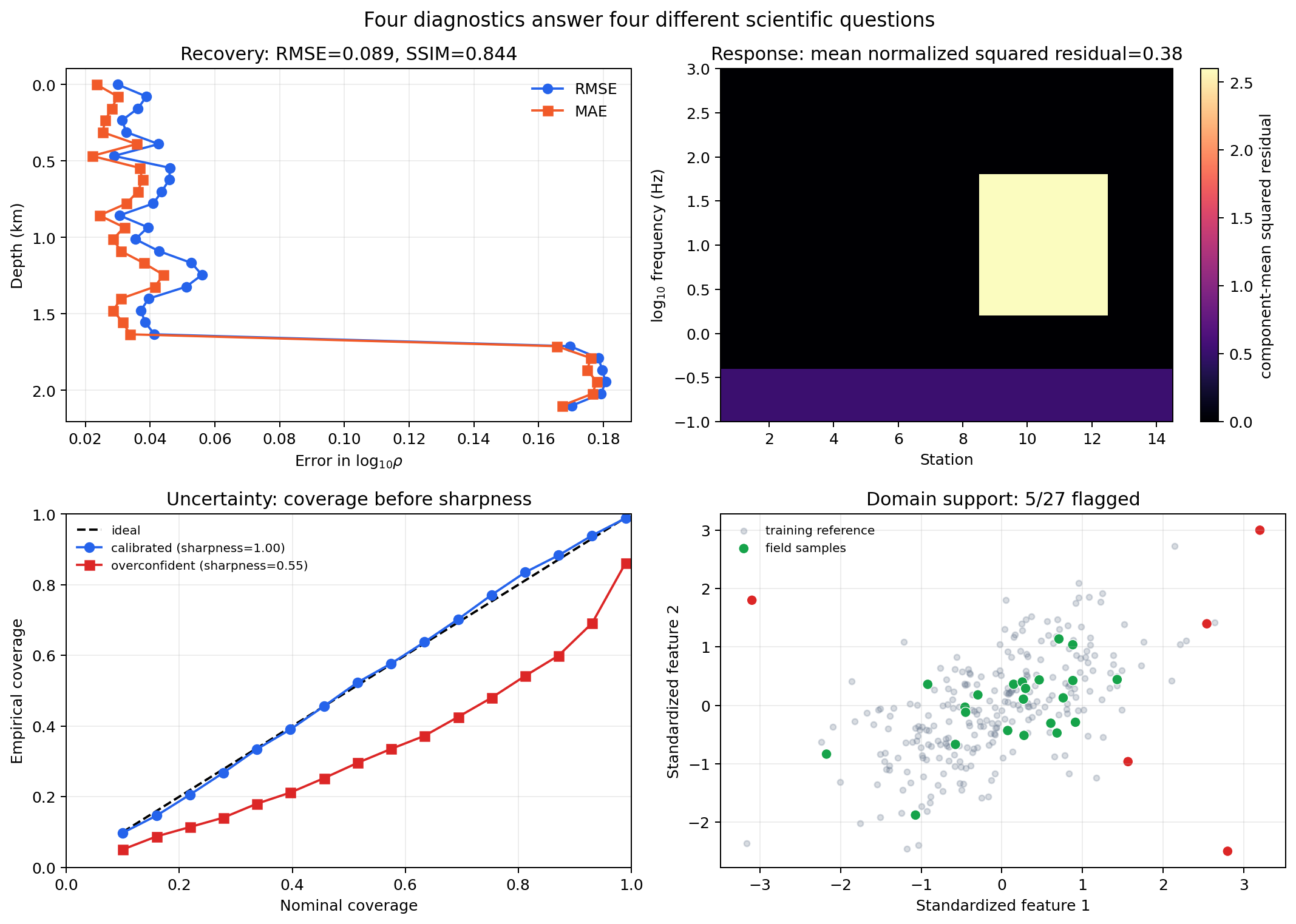
Synthetic recovery depth errors, response residual heat map, uncertainty reliability curves, and out-of-distribution feature screening — Four independent views of model recovery, response fit, uncertainty calibration, and training-domain support.#

The upper-left profile shows that the deeper bias increases both RMSE and MAE even though the section-wide SSIM remains high; structural similarity has not cancelled a depth-dependent amplitude error. The response heat map then localizes a different failure: a compact station-frequency block is poorly fit, while the lowest-frequency rows carry a smaller survey-wide mismatch. Neither pattern is recoverable from the global response mean alone.

In the lower-left panel, reducing predictive standard deviation makes the red model sharper but moves its reliability curve far below the diagonal. Its intervals are narrower because it is overconfident, not because it predicts better. Finally, the lower-right panel flags five feature vectors: the three visibly extreme points and two less obvious covariance-normalized departures. That is not a plotting error. Mahalanobis distance follows the reference covariance, so a point can look close in ordinary Euclidean distance while lying across a narrow direction of the reference ellipse. Green points are supported in these two selected features; they are not certified geologically correct. Taken together, the panels show why passing one diagnostic cannot compensate for failing another.

6.3.10.6. Turning diagnostics into an acceptance decision#

Validation becomes an acceptance test only after thresholds are frozen before examining the candidate result. AcceptanceCriterion provides that boundary; Reproducible experiment configuration explains how the criteria are stored with the complete experiment configuration. The metric mapping can be built directly from the immutable reports:

>>> from pycsamt.ai.experiments import AcceptanceCriterion

>>> criteria = (
...     AcceptanceCriterion("test.model_rmse", "<=", 0.20),
...     AcceptanceCriterion("test.response_msne", "<=", 2.00),
...     AcceptanceCriterion("test.calibration_mse", "<=", 0.01),
...     AcceptanceCriterion("field.ood_fraction", "<=", 0.10),
... )
>>> observed = {
...     "test.model_rmse": 0.1533,
...     "test.response_msne": 81.25,
...     "test.calibration_mse": 0.0002,
...     "field.ood_fraction": 0.04,
... }
>>> outcomes = {c.metric: c.evaluate(observed[c.metric]) for c in criteria}
>>> outcomes
{'test.model_rmse': True, 'test.response_msne': False, 'test.calibration_mse': True, 'field.ood_fraction': True}
>>> all(outcomes.values())
False

Three passing checks do not outvote the failed response criterion. The candidate is rejected because the gate is conjunctive, as formalized in (1). The numerical thresholds above demonstrate the API; they are not pyCSAMT defaults and must be justified from the survey’s error model, synthetic benchmark suite, and intended decision risk. In a real experiment, pass the same criteria to ExperimentConfig so missing metrics also make the gate incomplete rather than disappearing from the decision.

6.3.10.7. What actually reaches an agent’s result today#

recovery_report() is not only documented here — it already runs inside Inv2DAgent’s physics="mt2d" path. When a held-out synthetic test or validation partition is available, the agent predicts on it, compares against its known-truth resistivity with exactly this function, and folds the averaged RMSE/MAE/\(R^2\) into its result, precisely because a field survey has no ground truth to run the same check against — a synthetic partition is the only place this class of check can run at all. residuals, calibration, and ood are not wired into that same automatic result yet; they are available today the same way Loss functions for scientific inversion’s response, boundary, and uncertainty terms are — correct, tested, and ready to be called explicitly on a ForwardResult, SurveyData, or reference feature set, rather than produced automatically by every inversion run.