11.27.6. Learned Dimensionality Classification

classify_dimensionality() labels each (station, frequency) observation 1-D, 2-D, or 3-D from two thresholds on phase-tensor skew and ellipticity – transparent, but a hard boundary at a fixed skew value treats a sample just below the cutoff identically to one far below it, and ignores the other three phase-tensor-derived quantities that phase_features_table() already computes. DimensionalityClassifier is a multi-layer perceptron (MLP) trained on all five features at once – \([\,|\beta|,\ \text{ellipticity},\ \log_{10}\rho_{\det},\ \phi_{\det},\ |T|\,]\) – with two output heads sharing one backbone: a 3-class softmax for dimensionality, and a linear regression head for geoelectric strike on the 2-D subset.

11.27.6.1. Self-training from the rule-based labels

from_features_table() builds training labels from the same rule-based thresholds it is meant to refine when no label_col is supplied – the network’s job is not to invent a new definition of dimensionality, but to interpolate the rule-based boundary more smoothly across all five features jointly, rather than two features and a hard cutoff.

>>> from pycsamt.emtools.dimensionality import phase_features_table
>>> feats = phase_features_table(sites)
>>> len(feats), feats["station"].nunique()
(1484, 28)

Warning

The strike head is a separate branch that only receives gradient updates through its own loss term, added only when real strike targets are supplied via strike= (in fit()) or strike_col= (in from_features_table()). Call from_features_table(feats) with neither, as the self-training description above might suggest, and the strike head trains on nothing at all – predict_strike() still returns numbers, but they carry no information and should not be interpreted physically. Always supply real strike targets when the predicted strike matters, as done next.

11.27.6.2. Supervising the strike head with a classical estimate

estimate_strike_phase_tensor() computes one classical, per-station consensus strike angle from the same phase-tensor table. Broadcasting it back onto every frequency row of its station turns it into a real strike_col teacher signal – the strike-head counterpart of the rule-based dimensionality labels:

>>> from pycsamt.emtools.strike import estimate_strike_phase_tensor
>>> from pycsamt.ai.processing import DimensionalityClassifier
>>> consensus = estimate_strike_phase_tensor(sites)
>>> consensus[["station", "ang", "iqr"]].head(3)
  station        ang        iqr
0 18-001A -50.071764  28.974476
1 18-002U -43.757578  16.329767
2 18-003A -38.949283  18.993311
>>> feats = feats.merge(
...     consensus[["station", "ang"]], on="station", how="left",
... ).rename(columns={"ang": "strike_target"})
>>> clf = DimensionalityClassifier.from_features_table(
...     feats, strike_col="strike_target", epochs=120, seed=0,
...     verbose=False,
... )
DimensionalityClassifier(n_classes=3, torch, fitted)
>>> table = clf.predict_table(sites)
>>> table["dim_label"].value_counts()
3D    1368
2D     116
Name: count, dtype: int64
>>> n2d = int((table["dim"] == 1).sum())
>>> table.loc[table["dim"] == 1, "strike"].mean(), \
...     table.loc[table["dim"] == 1, "strike"].std()
(-42.9, 3.3)
>>> consensus["ang"].mean()
-39.4

Averaged over the 116 samples the network itself classified as 2-D, the predicted strike (\(-42.9^\circ \pm 3.3^\circ\)) lands within four degrees of the classical per-station consensus averaged over all 28 stations (\(-39.4^\circ\)) – direct evidence that the strike head learned a physically meaningful regression rather than collapsing to an arbitrary constant, which is precisely the failure mode the warning above describes for the unsupervised case.

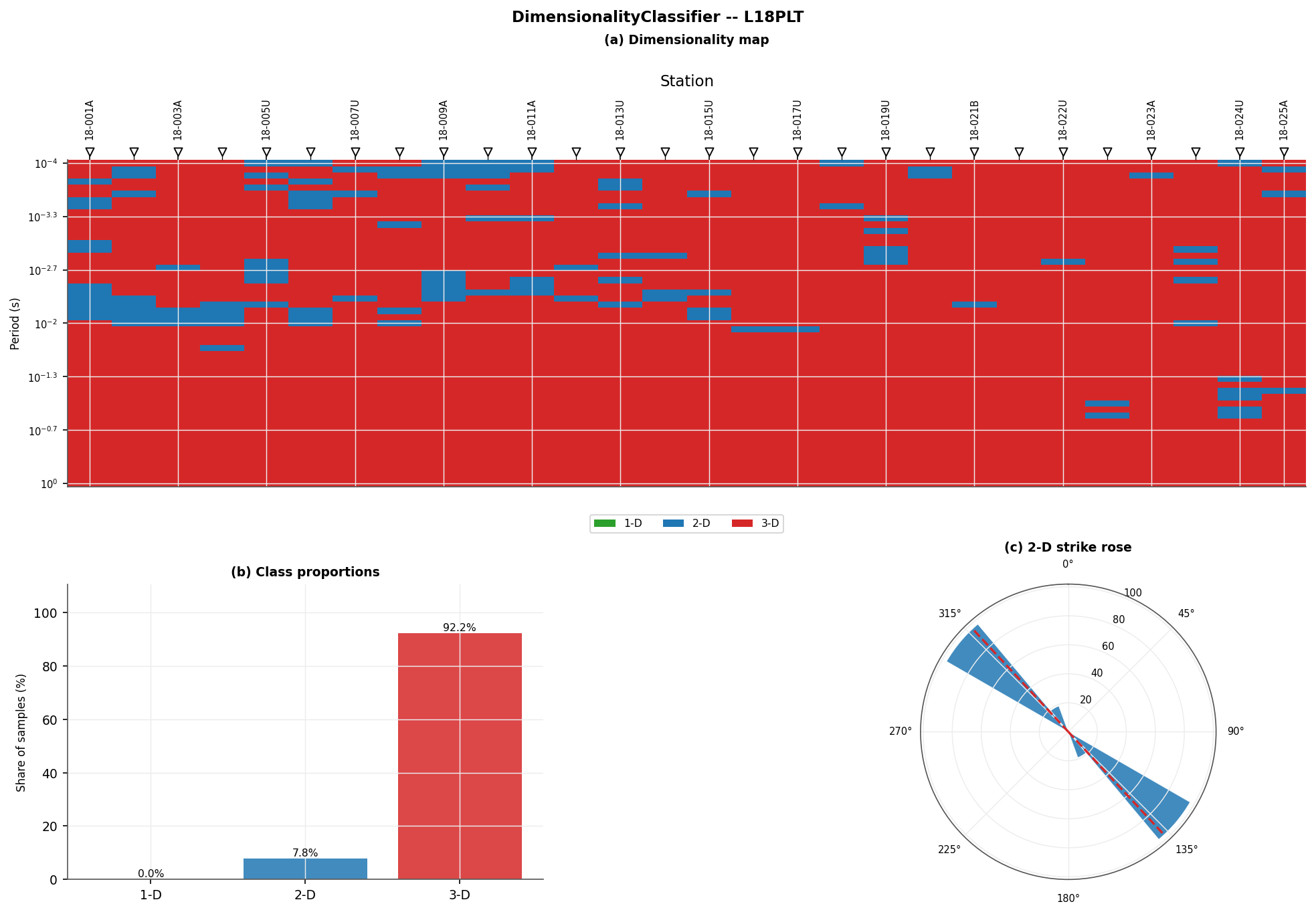
plot_dimensionality_summary() – the station x frequency class map, class proportions, and the 2-D strike rose (folded to the standard 180-degree line-ambiguity convention, with the circular mean overlaid as a dashed line).

L18PLT classifies as predominantly 3-D (92%), with a 2-D minority (8%) concentrated at short period along most of the line and a handful of long-period 2-D windows near the profile’s last few stations. This matches the picture built independently in Machine-Learning Quality Scoring: the stations whose median QC score collapsed under the hard skew rule are exactly the ones a genuinely 3-D subsurface response would be expected to produce. 1-D observations are rare in the rule-based training labels themselves – well under 5% of the L18PLT dataset – and this run predicted none at all, which is not a bug: with training labels this imbalanced, a self-trained network is not guaranteed to recover the minority class every time. If 1-D detection matters for your survey, check the raw rule-based label balance first and consider class weighting.

Note

The exact counts above will drift a little from run to run – DimensionalityClassifier’s PyTorch weight initialization is not seeded (the same caveat noted for AnomalyDetector in Profile-Level Anomaly Detection), so fit(seed=0) reproduces the data split exactly but not the network’s starting point. The qualitative picture – overwhelmingly 3-D, a real 2-D minority near short period, an unreliable 1-D minority, and a predicted strike within a few degrees of the classical consensus – is stable across runs even when the exact tallies are not.

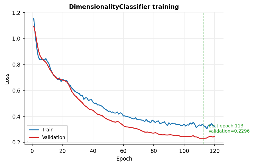
plot_training_history() – both curves report classification cross-entropy only, on the same scale, so they can be compared directly even though the strike MSE term also contributes to the gradient during training.

11.27.6.3. Parameters

hidden (default (128, 64)) sets the shared-backbone width; dropout (default 0.2) regularizes it. The strike loss weight is fixed at 0.1 relative to the classification cross-entropy, low enough that strike supervision refines the shared features without dominating the primary classification objective. Falls back to a random-forest classifier (scikit-learn) when neither PyTorch nor TensorFlow is installed – predict_strike() then always returns NaN, since the fallback has no regression head at all.

Full signatures: DimensionalityClassifier, phase_features_table(), estimate_strike_phase_tensor(), plot_dimensionality_map(), plot_predicted_strike_rose(), and plot_dimensionality_summary().

Note

plot_predicted_strike_rose() draws a rose from an already-computed array of predicted angles (as returned by predict_table()) and is intentionally distinct from plot_strike_rose(), which recomputes strike from a site collection using the classical estimators described in Geoelectric Strike.

</>View the complete DimensionalityClassifier example sourceClick to inspect and copy the complete code

def run_classify(sites, save_dir: Path) -> None:
    print("\n=== DimensionalityClassifier ===")
    feats = phase_features_table(sites)
    print(f"  feature rows: {len(feats)}")
    print(f"  stations: {feats['station'].nunique()}")

    # Classical, per-station phase-tensor strike (emtools.strike) supplies
    # the strike-head training target.  Without it, from_features_table's
    # default self-training path (rule-based dimensionality labels only)
    # never supervises the strike head at all -- see the note below.
    consensus = estimate_strike_phase_tensor(sites)
    feats = feats.merge(
        consensus[["station", "ang"]], on="station", how="left"
    ).rename(columns={"ang": "strike_target"})
    print("  classical (phase-tensor) strike per station -- head/tail:")
    print(
        consensus[["station", "ang", "iqr"]]
        .head(3)
        .to_string(index=False)
    )

    clf = DimensionalityClassifier.from_features_table(
        feats, strike_col="strike_target", epochs=120, seed=0,
        verbose=False,
    )
    print(f"  {clf!r}")
    hist = clf.history_
    if hist.get("val_loss"):
        print(f"  final val_loss: {hist['val_loss'][-1]:.5f}")

    table = clf.predict_table(sites)
    counts = table["dim_label"].value_counts()
    print("  predicted class counts:")
    print(counts.to_string())
    n2d = int((table["dim"] == 1).sum())
    if n2d:
        strike_mean = table.loc[table["dim"] == 1, "strike"].mean()
        strike_std = table.loc[table["dim"] == 1, "strike"].std()
        print(f"  predicted strike over {n2d} 2-D samples: "
              f"{strike_mean:.1f} +/- {strike_std:.1f} deg")
        print(f"  classical consensus (all stations): "
              f"{consensus['ang'].mean():.1f} deg")

    fig = plot_dimensionality_summary(
        table, suptitle="DimensionalityClassifier -- L18PLT"
    )
    _save(fig, save_dir, "dimensionality_summary.png")

    ax = plot_training_history(
        clf, title="DimensionalityClassifier training"
    )
    _save(ax.figure, save_dir, "dimensionality_training.png")

Point load_l18() at your own EDI folder to adapt this script