11.27.9. Learned Distortion Triage

pycsamt.emtools.ss already estimates static shift with four different spatial-statistics methods, and pycsamt.emtools.gb already fits a full Groom-Bailey galvanic-distortion decomposition by nonlinear least squares. DistortionTypeClassifier is not meant to replace either – it is meant to triage: given a station’s phase-tensor invariants and its already-fitted Groom-Bailey parameters, label it clean, static-shift-only, or genuinely distorted, the same way DimensionalityClassifier refines a threshold rule into a smoother multi-feature classifier rather than inventing a new definition of dimensionality. The value is routing a survey’s many stations toward the right existing tool quickly, not a new distortion model:

• clean – resistivity close to the along-line spatial trend, twist and shear close to 0; no correction needed.

• static-shift-only – resistivity departs from the trend but twist and shear stay small: a pure multiplicative offset, the case pycsamt.emtools.ss targets directly.

• distorted – twist and/or shear are non-negligible: rotation- and anisotropy-like distortion a static-shift correction alone cannot fix, the case apply_groom_bailey() targets.

11.27.9.1. Building the feature table

Each station is described by six numbers: \([\,|\beta|,\ \text{ellipticity},\ \Delta\log_{10}\rho,\ \text{twist},\ \text{shear},\ \text{anisotropy}\,]\). The first two come from phase_features_table() (median over frequency, already reused by DimensionalityClassifier); twist, shear, and anisotropy come from groom_bailey_table(), one real distortion matrix per station by construction.

Note

Groom-Bailey’s own fitted distortion matrix is normalised to unit determinant at every iteration – the textbook convention, since absolute gain is degenerate with the unknown regional resistivity and genuinely unrecoverable from one station’s data alone. Its gain column is therefore always exactly 1.0 and carries no information about static shift, even though it looks like exactly the number this page needs. \(\Delta\log_{10}\rho\), a real cross-station spatial comparison from estimate_ss_ama(), is used instead – found the same way the Learned Uncertainty Calibration page’s snr exclusion was: by checking a candidate feature’s actual behaviour against real data before trusting it, here discovering it was constant rather than a hidden copy of the target.

>>> from pycsamt.ai.processing import build_distortion_features_table
>>> from pycsamt.emtools import ensure_sites
>>> sites = ensure_sites("data/AMT/WILLY_DATA/L18PLT", recursive=True)
>>> feats = build_distortion_features_table(sites)
>>> feats.shape
(28, 7)
>>> feats[["delta_log10_rho", "twist_deg", "shear"]].describe().loc[
...     ["min", "max", "std"]
... ].round(3)
     delta_log10_rho  twist_deg  shear
min           -0.693    -56.802 -0.718
max            0.760     58.219  0.919
std            0.313     27.248  0.469

All three genuinely vary across a wide, physically meaningful range – twist alone spans ±57 degrees with a 27-degree standard deviation, confirming this survey has real galvanic rotation to triage, not a degenerate feature.

11.27.9.2. Self-training and a real limitation

from_features_table() builds default training labels from simple thresholds on \(|\text{twist}|\), \(|\text{shear}|\), and \(|\Delta\log_{10}\rho|\) when no real labels are supplied – the network’s job is to interpolate that rule-based boundary more smoothly across all six features jointly, the same self-training pattern Learned Dimensionality Classification uses. The rule-based labels themselves are fully deterministic:

>>> from pycsamt.ai.processing.distortion import _rule_labels
>>> import pandas as pd
>>> y_rule = _rule_labels(
...     feats["delta_log10_rho"].to_numpy(),
...     feats["twist_deg"].to_numpy(),
...     feats["shear"].to_numpy(),
... )
>>> pd.Series(y_rule).map(
...     {0: "clean", 1: "static_shift_only", 2: "distorted"}
... ).value_counts()
distorted            25
static_shift_only     3
Name: count, dtype: int64

Warning

The network’s predicted counts are far less stable than this rule-based reference, and not only in the usual “a minority class sometimes vanishes” sense already noted for Learned Dimensionality Classification and Profile-Level Anomaly Detection. With only 28 stations to self-train on and a 3-class split this imbalanced (25/3/0), repeated from_features_table(feats, epochs=80, seed=0) calls have been observed to disagree on which class is the majority: one run gave 25 distorted / 3 static-shift-only, matching the rule almost exactly; another gave 18 clean / 10 static-shift-only / 0 distorted – the opposite picture. Training longer narrows this but does not remove it: even at epochs=200, back-to-back runs have produced 27 distorted / 1 static-shift-only and, in the very next run, 26 static-shift-only / 2 distorted. seed only fixes the validation split, never PyTorch’s weight-initialization RNG (the same caveat as every other network-based estimator in this package – see Learned Spectral Denoising – but with consequences this visible only here, because 28 samples split three ways leaves very little signal for the loss to anchor on). Treat a single trained model’s predict_table output as one plausible smoothing of the rule boundary, not a converged answer – cross-check it against the rule-based labels above, train several seeds and compare, or supply real label_col labels when they are available. The run captured below happens to land close to the rule-based reference; your own run may not.

>>> from pycsamt.ai.processing import DistortionTypeClassifier
>>> clf = DistortionTypeClassifier.from_features_table(
...     feats, epochs=200, seed=0, verbose=False,
... )
>>> clf
DistortionTypeClassifier(n_classes=3, torch, fitted)
>>> table = clf.predict_table(sites)
>>> table[["station", "regime_label", "confidence"]].head(5)
  station       regime_label  confidence
0  18-001A          distorted    0.894951
1  18-002U          distorted    0.818244
2  18-003A  static_shift_only    0.420865
3  18-004A          distorted    0.824718
4  18-005U          distorted    0.768475
>>> table["regime_label"].value_counts()
regime_label
distorted            24
static_shift_only     4
Name: count, dtype: int64

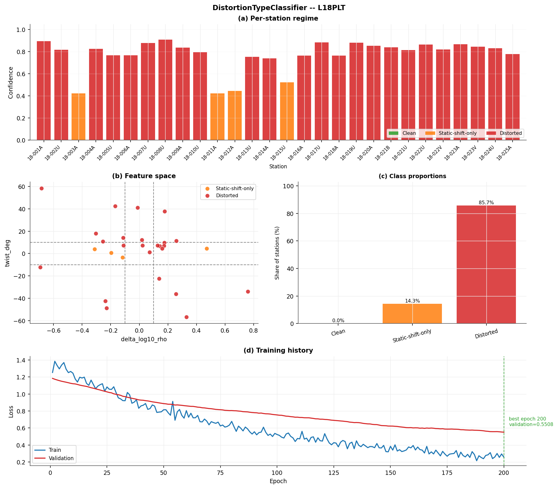
plot_distortion_summary() – (a) the per-station regime, bar colour for class and bar height for confidence; (b) the feature space that produced it, with the rule-based threshold lines overlaid; (c) class proportions, 85.7%/14.3%/0%, close to the rule-based 89.3%/10.7%/0% this run; (d) the training curve – still improving at epoch 200 (best epoch 200), the concrete evidence behind the undertraining warning above.

Panel (b) is worth reading closely even without a “clean” point on it this run: two of the four orange (static-shift-only) points sit close to, but on the correct side of, the vertical shift threshold, while the network’s decision for the borderline stations near the box corners can still disagree with a literal rule (only two of the three rule inputs are on this projection – a point can also cross the shear threshold, invisible here).

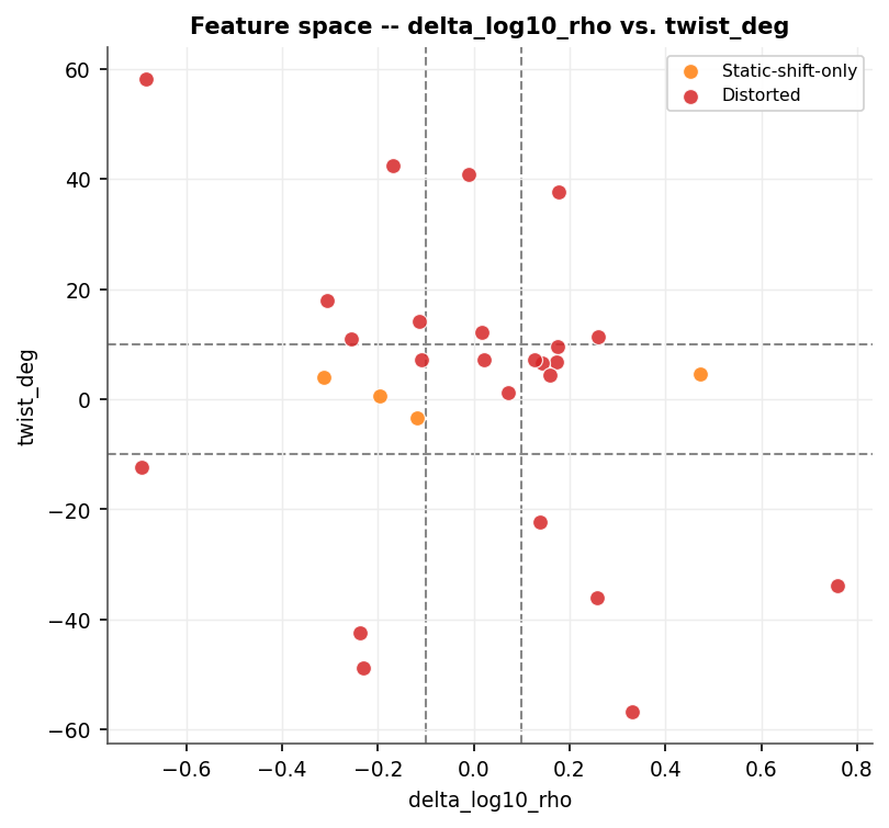
plot_distortion_feature_space() at full resolution – the same panel (b), standalone.

11.27.9.3. Routing to the real correction tools

The whole point of a triage classifier is to act on its output, not just report it. Splitting the site collection by predicted regime and handing each subset to the tool that regime actually calls for closes the loop:

>>> from pycsamt.emtools.gb import apply_groom_bailey
>>> from pycsamt.emtools.ss import correct_ss_ama
>>> ss_only = table.loc[
...     table["regime_label"] == "static_shift_only", "station"
... ].tolist()
>>> distorted = table.loc[
...     table["regime_label"] == "distorted", "station"
... ].tolist()
>>> len(ss_only), len(distorted)
(4, 24)
>>> ss_sites = sites.select(names=ss_only)
>>> ss_corrected = correct_ss_ama(ss_sites, inplace=False)
>>> len(list(ss_sites)), len(list(ss_corrected))
(4, 4)
>>> gb_sites = sites.select(names=distorted)
>>> gb_corrected = apply_groom_bailey(gb_sites, inplace=False)
>>> len(list(gb_sites)), len(list(gb_corrected))
(24, 24)

ss_corrected and gb_corrected are ordinary Sites collections – exactly what correct_ss_ama() and apply_groom_bailey() would return if called directly, since that is exactly what happened. No station was predicted “clean” on this particular run – when one is, it is simply left out of both subsets and untouched, since there is nothing to route it to.

11.27.9.4. Parameters and limitations

hidden (default (32, 16)) is deliberately smaller than Learned Dimensionality Classification’s default – this is a station-level problem (tens of samples per survey), not a station-frequency one. dropout (default 0.2) regularizes it. Given the instability documented above, prefer more epochs than the 80 default for anything beyond a quick look, and treat n_classes=3 labels from a single run as provisional.

Note

Falls back to a random-forest classifier (scikit-learn) when neither PyTorch nor TensorFlow is available; transform() then returns the forest’s own class probabilities.

Full signatures: DistortionTypeClassifier, build_distortion_features_table(), plot_distortion_map(), plot_distortion_feature_space(), and plot_distortion_summary().

</>View the complete DistortionTypeClassifier example sourceClick to inspect and copy the complete code

def run_distortion(sites, save_dir: Path) -> None:
    print("\n=== DistortionTypeClassifier ===")
    feats = build_distortion_features_table(sites)
    print(f"  station rows: {len(feats)}")
    print(f"  delta_log10_rho: min={feats['delta_log10_rho'].min():.3f} "
          f"max={feats['delta_log10_rho'].max():.3f} "
          f"std={feats['delta_log10_rho'].std():.3f}")
    print(f"  twist_deg: min={feats['twist_deg'].min():.1f} "
          f"max={feats['twist_deg'].max():.1f} "
          f"std={feats['twist_deg'].std():.1f}")
    print(f"  shear: min={feats['shear'].min():.3f} "
          f"max={feats['shear'].max():.3f} "
          f"std={feats['shear'].std():.3f}")

    from pycsamt.ai.processing.distortion import (
        _DISTORTION_LABELS,
        _rule_labels,
    )

    y_rule = _rule_labels(
        feats["delta_log10_rho"].to_numpy(),
        feats["twist_deg"].to_numpy(),
        feats["shear"].to_numpy(),
    )
    print("  rule-based label counts (deterministic self-training "
          "target):")
    import pandas as pd
    print(pd.Series([_DISTORTION_LABELS[i] for i in y_rule])
          .value_counts().to_string())

    clf = DistortionTypeClassifier.from_features_table(
        feats, epochs=200, seed=0, verbose=False,
    )
    print(f"  {clf!r}")
    hist = clf.history_
    if hist.get("val_loss"):
        best_ep = hist["val_loss"].index(min(hist["val_loss"])) + 1
        print(f"  final val_loss: {hist['val_loss'][-1]:.5f}, "
              f"best epoch: {best_ep}/{len(hist['val_loss'])}")

    table = clf.predict_table(sites)
    print(table[["station", "regime_label", "confidence"]]
          .head(5).to_string(index=False))
    print("  regime counts:")
    print(table["regime_label"].value_counts().to_string())

    fig = plot_distortion_summary(
        table, history=clf,
        suptitle="DistortionTypeClassifier -- L18PLT",
    )
    _save(fig, save_dir, "distortion_summary.png")

    ax = plot_distortion_feature_space(
        table, title="Feature space -- delta_log10_rho vs. twist_deg",
    )
    _save(ax.figure, save_dir, "distortion_feature_space.png")

    # Triage in action: route each regime to the real correction tool
    # the classifier is meant to point at, not a new one of its own.
    from pycsamt.emtools.gb import apply_groom_bailey
    from pycsamt.emtools.ss import correct_ss_ama

    ss_only = table.loc[
        table["regime_label"] == "static_shift_only", "station"
    ].tolist()
    distorted = table.loc[
        table["regime_label"] == "distorted", "station"
    ].tolist()
    print(f"  routed to correct_ss_ama (static_shift_only): {len(ss_only)}")
    print(f"  routed to apply_groom_bailey (distorted): {len(distorted)}")

    if ss_only:
        ss_sites = sites.select(names=ss_only)
        ss_corrected = correct_ss_ama(ss_sites, inplace=False)
        print(f"  correct_ss_ama: {len(list(ss_sites))} -> "
              f"{len(list(ss_corrected))} stations corrected")

    if distorted:
        gb_sites = sites.select(names=distorted)
        gb_corrected = apply_groom_bailey(gb_sites, inplace=False)
        print(f"  apply_groom_bailey: {len(list(gb_sites))} -> "
              f"{len(list(gb_corrected))} stations corrected")

Point load_l18() at your own EDI folder to adapt this script