11.27.7. Learned Gap Filling#

Learned Spectral Denoising assumes every (station, frequency) cell has some value and improves its quality. Real surveys also have cells with no value at all – a frequency dropped mid-acquisition, a component that never converged, a band skipped for poor coherence – and nothing else in pyCSAMT fills those gaps with anything better than carrying NaN straight through to inversion. EMImputer targets that gap directly: reconstructing the missing cells from the observed ones using spectral smoothness – the same station, nearby frequencies – a matrix-completion problem, not a denoising one.

The recipe is the masked-reconstruction family, the same idea behind BERT-style masked-language modelling or image inpainting:

(1)#\[\hat{\mathbf{x}} = f_\theta(\mathbf{x} \odot \mathbf{m},\ \mathbf{m}), \qquad \mathcal{L} = \frac{\big\| (\hat{\mathbf{x}} - \mathbf{x}) \odot \mathbf{m}_\text{syn} \big\|_2^2}{\sum \mathbf{m}_\text{syn}}\]

where \(\mathbf{m} \in \{0, 1\}\) is the mask fed to the network (1 = “this cell is observed”) and \(\mathbf{m}_\text{syn}\) marks the subset of genuinely observed cells synthetically hidden on that training step – exactly where the loss is evaluated. On every step, fit() hides a random mask_frac fraction of the truly-observed cells (any real NaN gaps already in the training data are always hidden and never used as a target, since their true value is unknown), mirroring the way EMDenoiser adds synthetic noise. Training data therefore only needs to be mostly complete, not to come with real missing-data examples of known ground truth.

The network is the same 1-D convolutional encoder-decoder family as EMDenoiser, with one structural difference: the encoder takes 2 * n_components input channels – the zeroed-where-hidden values, concatenated with the observed-cell mask along the channel axis – so it can distinguish “zero because hidden” from “zero because that is genuinely the value”, while the decoder still only reconstructs n_components channels; the mask itself is never reconstructed.

11.27.7.1. A survey with real gaps#

L18PLT, used throughout the rest of this section, has no genuinely missing cells to fill – every earlier page here either works with complete data or synthesises noise on top of it. This page instead uses data/MT/broken-hill: 21 real “ultra-wide-band” magnetotelluric soundings recorded by the University of Sydney around the Broken Hill Pb-Zn-Ag deposit, New South Wales (AlQahtani et al., 2026, open-access CC-BY). Several of its stations really do have missing frequency rows – dropped estimates, most likely from reduced coherence at the long-period end of a station’s recording, where a wideband instrument has proportionally less time to average down noise.

>>> from pycsamt.ai.processing import EMImputer, prepare_z_features
>>> from pycsamt.emtools import ensure_sites
>>> sites = ensure_sites("data/MT/broken-hill/edis", recursive=True)
>>> X = prepare_z_features(sites, n_components=4)
>>> X.shape
(21, 4, 96)
>>> import numpy as np
>>> missing = np.isnan(X).any(axis=1)   # (n_sites, n_freqs)
>>> int(missing.sum())
43

prepare_z_features resamples every station onto one common frequency grid (freq_ref, the first site’s own grid by default) – 43 (station, frequency) rows come out with at least one NaN component after that resampling, spread across 5 of the 21 stations:

>>> per_site = missing.sum(axis=1)
>>> from pycsamt.emtools._core import _iter_items, _name
>>> labels = [_name(ed, i) for i, ed in enumerate(_iter_items(sites))]
>>> {labels[i]: int(per_site[i]) for i in range(len(labels))
...  if per_site[i] > 0}
{'BH_11_imp': 18, 'BH_19_imp': 10, 'BH_1_imp': 3, 'BH_4_imp': 9, 'BH_5_imp': 3}

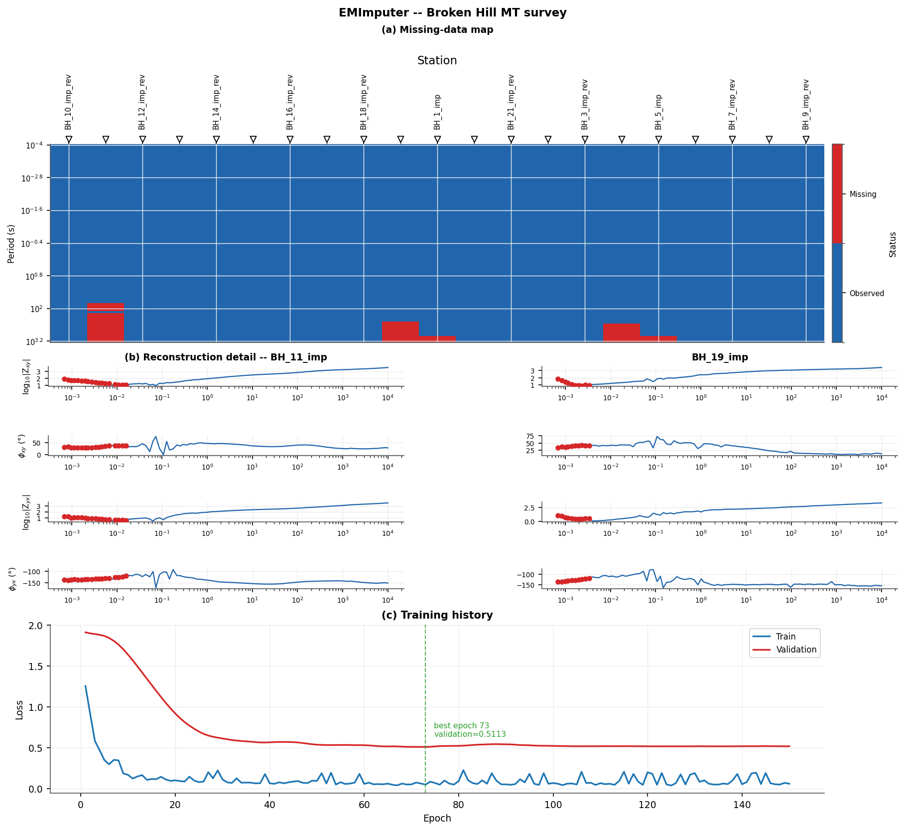
../../_images/imputer_summary.png — `plot_imputer_summary()` – (a) the station x frequency missing-data map (note the gaps cluster almost entirely at long period, consistent with the coherence explanation above); (b) two of the five gapped stations, filled curve in blue with reconstructed cells marked in red; (c) the training curve.#

11.27.7.2. Quantitative validation on held-out cells#

A genuinely missing cell has no known value to check a reconstruction against, so the standard masked-reconstruction validation protocol does the opposite of what a real gap is: it hides a known fraction of the already observed cells, reconstructs them, and compares the reconstruction to the real, held-back values.

>>> rng = np.random.default_rng(0)
>>> observed = np.isfinite(X)
>>> holdout = (rng.random(X.shape) < 0.12) & observed
>>> X_holdout = X.copy()
>>> X_holdout[holdout] = np.nan
>>> int(holdout.sum())
963
>>> imp = EMImputer(channels=(32, 64, 32))
>>> imp.fit(X_holdout, mask_frac=0.15, epochs=150, seed=0, verbose=False)
EMImputer(n_freqs=96, n_components=4, fitted)
>>> X_recon = imp.transform(X_holdout)
>>> y_true, y_pred = X[holdout], X_recon[holdout]

Warning

As with every network-based estimator in this package, seed fixes the held-out split and the synthetic training mask but not PyTorch’s own weight-initialization RNG – rerunning the block above reproduces the same protocol, not bit-identical numbers. See the equivalent caveat in Learned Spectral Denoising.

A single pooled RMSE across all four feature channels would repeat the mistake Learned Spectral Denoising warns about: log-amplitude and degree-valued phase channels sit on completely different scales, and whichever one has the larger numeric range would dominate. Broken down by channel against a channel-mean “predict nothing” baseline, every channel improves substantially:

Channel	n cells	RMSE, EMImputer	RMSE, baseline
\(\log_{10}\|Z_{xy}\|\)	234	0.179	0.978
\(\phi_{xy}\) (deg)	215	8.098	16.480
\(\log_{10}\|Z_{yx}\|\)	279	0.182	1.026
\(\phi_{yx}\) (deg)	235	6.081	17.983

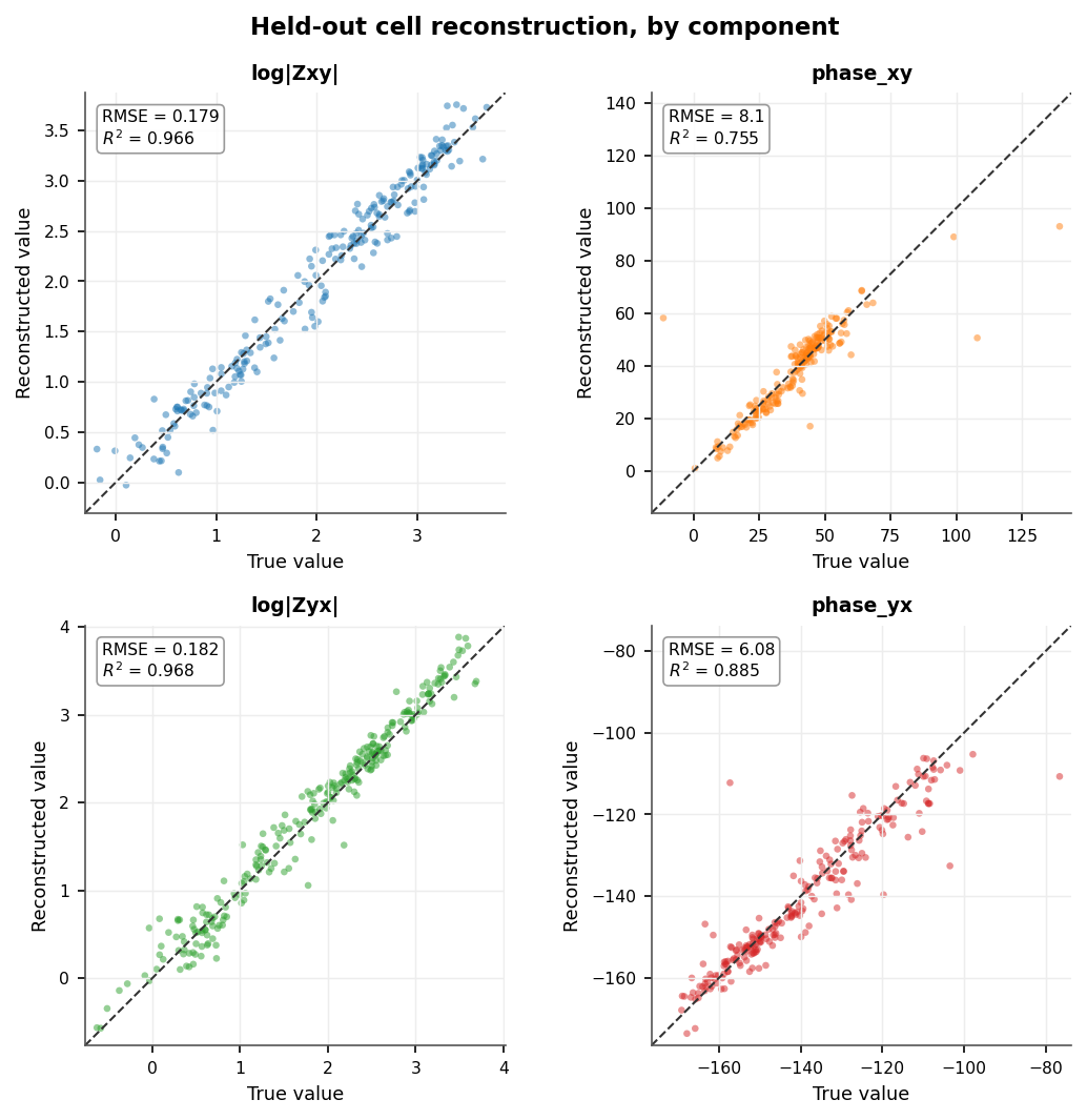
../../_images/imputer_validation.png — `plot_imputer_validation()`, one panel per feature component – true value on the x-axis, reconstructed value on the y-axis, dashed line at \(y = x\). Both log-amplitude channels track the diagonal closely (\(R^2\) 0.966 and 0.968); the phase channels are noisier but still clearly informative (\(R^2\) 0.755 and 0.885), consistent with phase generally being the harder quantity to reconstruct from neighbouring frequencies alone.#

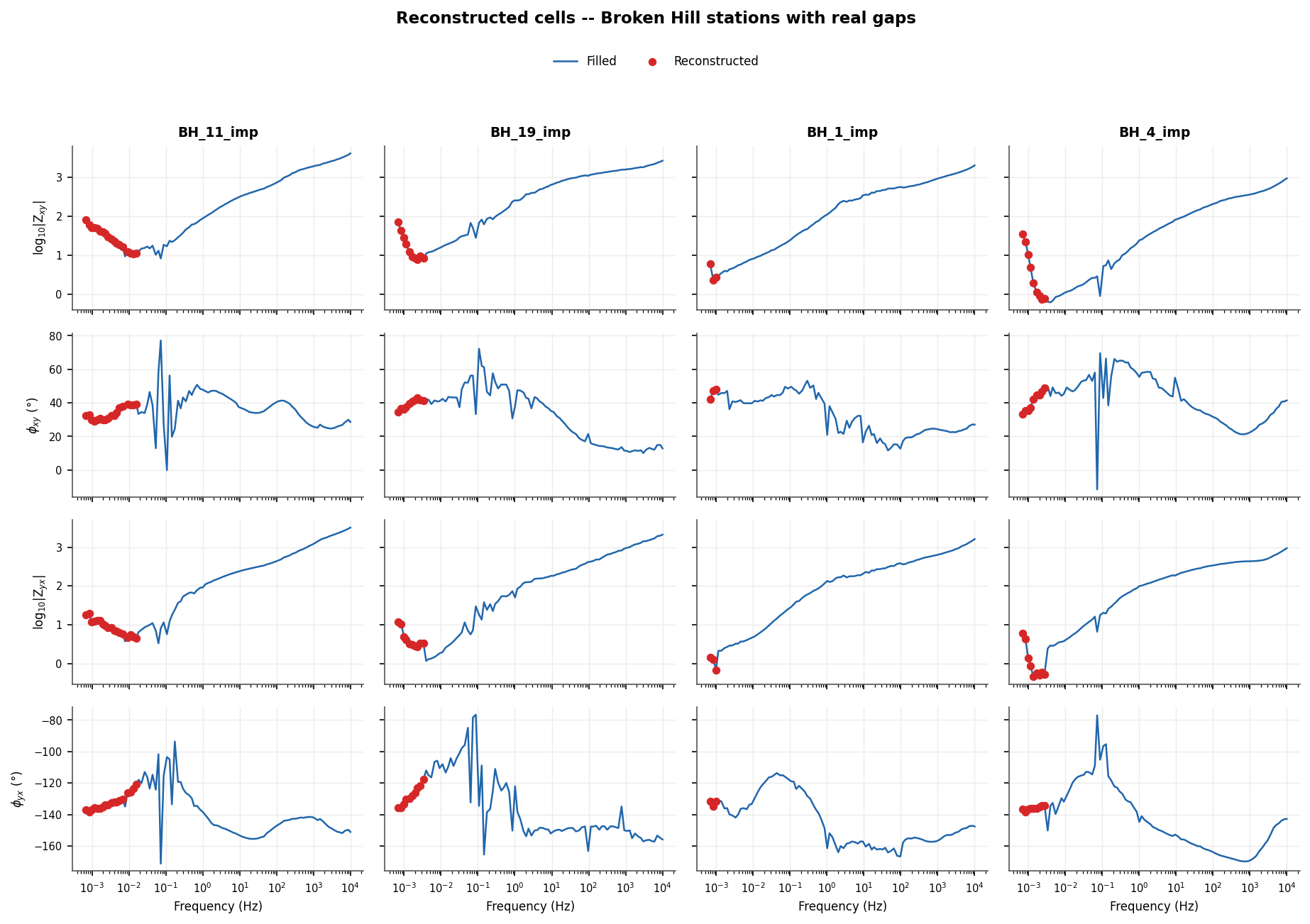
../../_images/imputer_reconstruction.png — `plot_imputer_reconstruction()` at full resolution for the four most-gapped stations. The reconstructed points (red) sit smoothly on the continuation of each curve’s real, observed trend rather than jumping off it – direct visual evidence that the network is extrapolating the station’s own spectral shape, not producing arbitrary values.#

11.27.7.3. Sites in, filled sites out#

apply() closes the same sites-in / sites-out loop as Learned Spectral Denoising’s apply(): pass a site collection, get one back, with an inplace flag controlling whether the input is mutated. The version fitted here trains on the full array – the real gaps stay NaN and excluded from the loss, none of the synthetic held-out cells from the validation above are involved:

>>> imp = EMImputer(channels=(32, 64, 32))
>>> imp.fit(X, mask_frac=0.15, epochs=150, seed=0, verbose=False)
EMImputer(n_freqs=96, n_components=4, fitted)
>>> filled_sites = imp.apply(sites, inplace=False)

Checking station BH_11_imp directly confirms both halves of that contract: every cell that was already observed comes back unchanged, and every genuinely missing row now has a reconstructed value.

>>> from pycsamt.emtools._core import _get_z_block
>>> gi = labels.index("BH_11_imp")
>>> ed_in = list(_iter_items(sites))[gi]
>>> ed_out = list(_iter_items(filled_sites))[gi]
>>> _, z_in, _ = _get_z_block(ed_in, with_errors=False)[:3]
>>> _, z_out, _ = _get_z_block(ed_out, with_errors=False)[:3]
>>> obs = ~np.isnan(z_in).any(axis=(1, 2))
>>> bool(np.allclose(z_in[obs], z_out[obs], equal_nan=True))
True
>>> was_missing = np.isnan(z_in).any(axis=(1, 2))
>>> int((was_missing & ~np.isnan(z_out[:, 0, 1])
...      & ~np.isnan(z_out[:, 1, 0])).sum())
20

Every observed cell in BH_11_imp is untouched, and all 20 of its missing rows now have \(Z_{xy}\) and \(Z_{yx}\) filled.

Warning

With the default n_components=4, only \(Z_{xy}\) and \(Z_{yx}\) are modelled – a real missing measurement usually means the whole frequency row (all four components) is absent, and the diagonal \(Z_{xx}, Z_{yy}\) at those rows is left exactly as it was, NaN if it was NaN, the same “not modelled -> untouched” contract apply() uses. Fit and apply with n_components=8 to fill every component.

11.27.7.4. Parameters and limitations#

mask_frac (default 0.15) controls how much of the observed data is hidden on every training step – too low and the network sees little missing-data signal to learn from; too high and too little context remains around a hidden cell for it to reconstruct anything. channels sets the encoder/decoder width at each stage, narrowed to (32, 64, 32) above for a 21-station survey the same way Learned Spectral Denoising narrows it for L18PLT. n_components (4 or 8) trades model complexity against diagonal-component coverage, as shown above.

Note

When neither PyTorch nor TensorFlow is installed, EMImputer falls back to per-sample, per-channel linear interpolation along the frequency axis – no cross-station information, unlike the network path, and a channel with no observed value anywhere in the training batch falls back further still, to that channel’s training mean.

Full signatures: EMImputer, prepare_z_features(), plot_imputer_gaps(), plot_imputer_validation(), plot_imputer_reconstruction(), and plot_imputer_summary().

View the complete EMImputer example sourceClick to inspect and copy the complete code

def run_imputer(sites, save_dir: Path) -> None:
    print("\n=== EMImputer ===")
    labels = station_names(sites)
    X = prepare_z_features(sites, n_components=4)
    n_sites, _n_comp, n_freq = X.shape
    print(f"  X shape: {X.shape}")

    from pycsamt.emtools._core import _get_z_block, _iter_items

    freq = None
    for ed in _iter_items(sites):
        result = _get_z_block(ed, with_errors=False)
        freq = result[2] if len(result) >= 3 else None
        if freq is not None:
            break

    missing_mask = ~np.isfinite(X)
    row_missing = missing_mask.any(axis=1)  # (n_sites, n_freq)
    per_site = row_missing.sum(axis=1)
    gapped = [
        (labels[i], int(per_site[i]))
        for i in range(n_sites)
        if per_site[i] > 0
    ]
    print(f"  genuinely missing rows: {int(row_missing.sum())} "
          f"across {len(gapped)} / {n_sites} stations")
    for name, n in gapped:
        print(f"    {name}: {n} missing rows (of {n_freq})")

    gap_table = pd.DataFrame(
        {
            "station": np.repeat(labels, n_freq),
            "freq": np.tile(freq, n_sites),
            "missing": row_missing.astype(int).ravel(),
        }
    )

    # Quantitative validation: real gaps have no known ground truth, so
    # hold out a random 12% of the *genuinely observed* cells instead
    # (seeded), fit with them additionally hidden, then compare the
    # reconstruction against the real, known values at those cells.
    rng = np.random.default_rng(0)
    observed = np.isfinite(X)
    holdout = (rng.random(X.shape) < 0.12) & observed
    X_holdout = X.copy()
    X_holdout[holdout] = np.nan
    print(f"  held-out cells for validation: {int(holdout.sum())}")

    imp_val = EMImputer(channels=(32, 64, 32))
    imp_val.fit(
        X_holdout, mask_frac=0.15, epochs=150, seed=0, verbose=False
    )
    X_recon_holdout = imp_val.transform(X_holdout)
    y_true = X[holdout]
    y_pred = X_recon_holdout[holdout]
    rmse_model = float(np.sqrt(np.mean((y_true - y_pred) ** 2)))

    chan_mean = np.nanmean(X_holdout, axis=(0, 2), keepdims=True)
    y_pred_naive = np.broadcast_to(chan_mean, X.shape)[holdout]
    rmse_naive = float(np.sqrt(np.mean((y_true - y_pred_naive) ** 2)))
    print(f"  RMSE (EMImputer), pooled:     {rmse_model:.4f}")
    print(f"  RMSE (channel-mean baseline): {rmse_naive:.4f}")
    print("  (pooled RMSE mixes log-amplitude and degree-valued phase "
          "channels -- see per-channel breakdown below)")

    comp_ids = np.broadcast_to(
        np.arange(X.shape[1])[None, :, None], X.shape
    )[holdout]
    for ci, name in enumerate(
        ["log|Zxy|", "phase_xy", "log|Zyx|", "phase_yx"]
    ):
        cm = comp_ids == ci
        rm = float(np.sqrt(np.mean((y_true[cm] - y_pred[cm]) ** 2)))
        rb = float(
            np.sqrt(np.mean((y_true[cm] - y_pred_naive[cm]) ** 2))
        )
        print(f"    {name:>9s} (n={int(cm.sum())}): "
              f"RMSE model={rm:.3f}  baseline={rb:.3f}")

    # The deployed imputer: fit on the full array (only the genuine
    # gaps are NaN -- none of the synthetic holdout above), then fill
    # those real gaps via apply().
    imp = EMImputer(channels=(32, 64, 32))
    imp.fit(X, mask_frac=0.15, epochs=150, seed=0, verbose=False)
    print(f"  {imp!r}")
    hist = imp.history_
    if hist.get("val_loss"):
        print(f"  final val_loss: {hist['val_loss'][-1]:.5f}")

    X_filled = imp.transform(X)
    filled_sites = imp.apply(sites, inplace=False)

    # Verify: observed cells byte-identical, gapped station now filled.
    gap_name = gapped[0][0] if gapped else labels[0]
    gi = labels.index(gap_name)
    for i, (ed_in, ed_out) in enumerate(
        zip(_iter_items(sites), _iter_items(filled_sites))
    ):
        if i != gi:
            continue
        _, z_in, _fr_in = _get_z_block(ed_in, with_errors=False)[:3]
        _, z_out, _fr_out = _get_z_block(ed_out, with_errors=False)[:3]
        obs = ~np.isnan(z_in).any(axis=(1, 2))
        same_observed = bool(
            np.allclose(z_in[obs], z_out[obs], equal_nan=True)
        )
        was_missing = np.isnan(z_in).any(axis=(1, 2))
        offdiag_filled = int(
            (
                was_missing
                & ~np.isnan(z_out[:, 0, 1])
                & ~np.isnan(z_out[:, 1, 0])
            ).sum()
        )
        diag_still_nan = int(
            (
                was_missing
                & (np.isnan(z_out[:, 0, 0]) | np.isnan(z_out[:, 1, 1]))
            ).sum()
        )
        print(f"  {gap_name}: observed rows unchanged = {same_observed}; "
              f"of {int(was_missing.sum())} missing rows, "
              f"{offdiag_filled} now have Zxy/Zyx filled, "
              f"{diag_still_nan} still have Zxx/Zyy = NaN "
              f"(n_components=4 -> diagonal not modelled)")
        break

    fig = plot_imputer_summary(
        gap_table, freq, X, X_filled,
        history=imp, station_labels=labels,
        n_show=2,
        suptitle="EMImputer -- Broken Hill MT survey",
    )
    _save(fig, save_dir, "imputer_summary.png")

    show_idx = [labels.index(n) for n, _ in gapped[:4]] or [0]
    fig = plot_imputer_reconstruction(
        freq, X, X_filled, station_labels=labels, sites=show_idx,
        suptitle="Reconstructed cells -- Broken Hill stations with real gaps",
    )
    _save(fig, save_dir, "imputer_reconstruction.png")

    fig = plot_imputer_validation(
        y_true, y_pred, component_ids=comp_ids,
        component_labels=["log|Zxy|", "phase_xy", "log|Zyx|", "phase_yx"],
        suptitle="Held-out cell reconstruction, by component",
    )
    _save(fig, save_dir, "imputer_validation.png")

Point load_broken_hill() at your own EDI folder to adapt this script