11.27.4. Raw Time-Series Denoising (MMF-SVM-K-SVD)#

Every other tool in this section works downstream of an already-computed impedance tensor. EMDenoiser (Learned Spectral Denoising) smooths a spectrum; notch_powerline() and its neighbours correct known, structured artefacts in \(Z\). Neither can help with strong, non-stationary interference that is already baked into the impedance estimate before either tool ever sees the data – a charge/discharge transient, a square-wave step from a nearby power line, an isolated pulse – because by the time ts_to_spectra() has Fourier-transformed a contaminated segment, the interference’s energy has spread across every frequency band the segment contributes to. TimeSeriesDenoiser works one stage further upstream, directly on the raw TSData sample stream that read_ts() produces – the same object preprocess()’s light gap-fill and cross_spectra()’s Huber-robust segment weighting already work with, just before either of them runs.

The method is a direct implementation of Gui et al. (2024) [Gui2024], extending the same authors’ earlier MMF-K-SVD approach [Gui2021] with a classification stage that stops a naive denoiser from quietly deleting genuine, low-amplitude MT signal along with the interference. Three stages run in sequence:

Mathematical morphological filtering (MMF) splits each channel into a low-frequency envelope, kept untouched, and a high-frequency residual that may carry strong interference.
A support vector machine (SVM) classifies each window of that residual as clean or noisy from four complexity features.
K-SVD dictionary learning denoises only the windows the SVM flagged, leaving classified-clean windows – and the untouched low-frequency envelope – exactly as recorded.

Separating low frequencies before anything else matters because MT signal is overwhelmingly low-frequency, and a global decomposition such as CEEMD, VMD, or a wavelet transform loses its footing exactly where a strong transient corrupts the envelope it is trying to extract [Gui2024]. MMF, first applied to MT sounding data by [Tang2012], sidesteps that failure mode by working locally in time rather than fitting a global basis: it separates a channel \(x\) into a low-frequency envelope and a high-frequency residual via grayscale erosion (\(\epsilon_g\)) and dilation (\(\delta_g\)) with a flat structuring element of length \(L\) samples,

(1)#\[x_{low} = \tfrac{1}{2}\left[\mathrm{OC}(x) + \mathrm{CO}(x)\right], \qquad \mathrm{OC}(x) = \delta_g\big(\epsilon_g(x)\big), \quad \mathrm{CO}(x) = \epsilon_g\big(\delta_g(x)\big),\]

with \(x_{high} = x - x_{low}\). Averaging the “open-then-close” and “close-then-open” orderings removes both positive and negative transients symmetrically – a spike that survives one ordering is suppressed by the other. \(L\) (the size argument of mmf_split(), in samples) is the parameter that matters most, and it is unavoidably data-dependent: it must exceed the widest interference pulse in the record, or that pulse’s plateau survives erosion and dilation intact and leaks straight into \(x_{low}\) instead of being rejected into \(x_{high}\) where the next two stages can deal with it. A real ~580-unit burst in EY from pyCSAMT’s bundled long-period recording data/MT/TS/kap103as.ts (introduced fully below) makes the effect concrete:

>>> from pycsamt.ai.processing import mmf_split
>>> for size in (31, 61, 121, 241, 361):
...     low, _ = mmf_split(ey_burst, size=size)
...     print(size, low.min(), low.max())
31   -4.46  59.67
61   -4.12  37.86
121  -3.45  19.57
241  -1.83   5.89
361  -0.15   3.43

As \(L\) grows from 31 samples (155 s) to 361 samples (1805 s), the leaked amplitude in low shrinks steadily from nearly 60 units down to 3.4 – close to the channel’s own quiet-period background. Left at its automatic default (size=None, roughly 2 s worth of samples), mmf_split() would be far too narrow for a burst this wide and would leave most of it sitting uncorrected in the low-frequency output. Plotting the well-tuned split (\(L=241\)) makes the payoff visible directly:

>>> from pycsamt.ai.processing import plot_ts_denoise_mmf_split
>>> t = np.arange(ey_burst.size) * dt   # dt = 5.0 s for this station
>>> low, high = mmf_split(ey_burst, size=241)
>>> plot_ts_denoise_mmf_split(t, ey_burst, low, high)

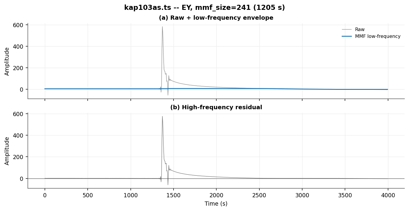
../../_images/tsdenoise_mmf_split_real.png — `plot_ts_denoise_mmf_split()` for the real `kap103as.ts` burst at \(L=241\). (a) the raw channel with its MMF envelope overlaid – flat at essentially zero through the entire burst; (b) the high-frequency residual, which now carries almost the whole burst amplitude rather than a fraction of it.#

Warning

mmf_split()’s size=None default assumes a sampling rate on the order of the paper’s own 15 Hz CSAMT-style acquisition, where a handful of seconds is already several dozen samples. It is a poor default for long-period MT (kap103’s 5 s sampling above) or for any record where interference bursts last minutes rather than seconds – pass size (or the equivalent mmf_size on TimeSeriesDenoiser) explicitly rather than trusting the default on unfamiliar data.

11.27.4.1. Separating signal from noise with a support vector machine#

Once the high-frequency residual is isolated, it is cut into win_seconds-long windows and each one is classified clean or noisy. A support vector machine finds the hyperplane that maximises the margin between the two classes in feature space – effective here with very little training data because the feature set is small (four numbers per window) and the classes are, in practice, well separated. The four features are complexity measures: sample entropy, fuzzy entropy, and approximate entropy [Richman2000] [Pincus1995] [Chen2007] all compare how often short embedded subsequences that match within a tolerance \(r\) continue to match one sample further,

(2)#\[\mathrm{SampEn}(m, r) = -\ln\frac{A}{B},\]

where \(B\) counts length-\(m\) template matches (excluding self-matches) and \(A\) counts length-\((m+1)\) matches under the same tolerance – large for an irregular, weak-amplitude, strongly random signal (genuine MT background) and small for a stereotyped, repeated shape (a charge/discharge or square-wave transient). The fourth feature, box-counting dimension, measures the same regular-vs-ragged contrast geometrically rather than statistically. compute_entropy_features() computes all four at once, for as many windows as its input has rows:

>>> from pycsamt.ai.processing import compute_entropy_features
>>> clean_window = high[0:60]              # no injected transient
>>> burst_window = high[600:660]           # charge/discharge burst
>>> square_window = high[1200:1260]        # square block
>>> for name, w in [("clean", clean_window), ("burst", burst_window),
...                 ("square", square_window)]:
...     se, fe, ae, bd = compute_entropy_features(w[None, :])[0]
...     print(f"{name:>7s}  SE={se:.3f} FE={fe:.3f} AE={ae:.3f} BD={bd:.3f}")
  clean  SE=1.856 FE=1.754 AE=0.462 BD=1.179
  burst  SE=0.309 FE=0.273 AE=0.242 BD=1.097
 square  SE=0.169 FE=0.185 AE=0.201 BD=0.985

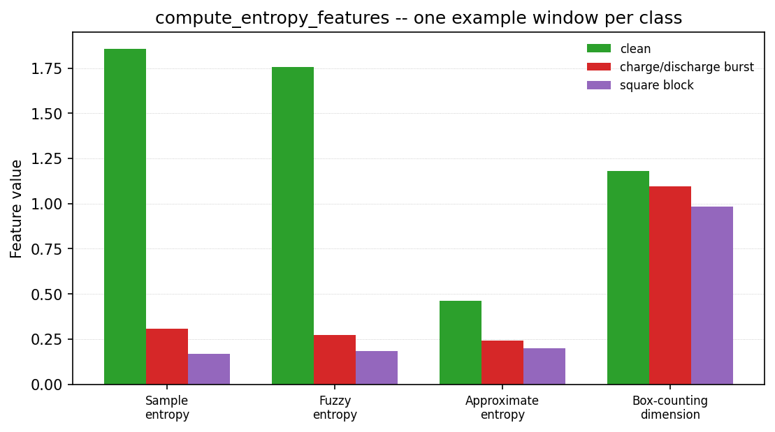
../../_images/tsdenoise_entropy_features.png — The four features above, one example window per class. All four drop from the clean window to both interference windows, box-counting dimension by the smallest margin (it captures the same regular-vs-ragged contrast geometrically, with less separation power here than the three entropy measures) – a pattern that echoes Fig. 4 of Gui et al. (2024).#

generate_synthetic_library() builds a labelled training library by pairing the same weak, band-limited colored-noise background used throughout this page with one of four interference shapes – charge/discharge, square, pulse, triangle – mirroring the sample library Gui et al. (2024) built from real strong-interference and high-quality segments (their Fig. 3). SignalQualityClassifier wraps a linear-kernel sklearn.svm.SVC around this feature vector:

>>> import numpy as np
>>> from pycsamt.ai.processing import (
...     SignalQualityClassifier, generate_synthetic_library,
... )
>>> segs, y = generate_synthetic_library(win_len=60, n_per_class=150, seed=11)
>>> rng = np.random.default_rng(12)
>>> idx = rng.permutation(len(segs))
>>> n_train = int(0.7 * len(segs))
>>> tr, te = idx[:n_train], idx[n_train:]
>>> clf = SignalQualityClassifier(random_state=0).fit(segs[tr], y[tr])
>>> pred = clf.predict(segs[te])
>>> float((pred == y[te]).mean())
0.9333

93% holdout accuracy across all four interference shapes, from a 150-samples-per-class synthetic library and a linear kernel, echoes the clean separation Fig. 6 of Gui et al. (2024) reports for their own measured-data test set – consistent with \(\mathrm{SampEn}\) and its relatives genuinely capturing a robust, shape-independent contrast between regular interference and random background, not an artefact of one particular noise type.

Applied to a whole record rather than one window at a time, plot_ts_denoise_segments() shows the classification stage on its own – before K-SVD does anything – shading every window the SVM called noisy directly on the MMF high-frequency residual:

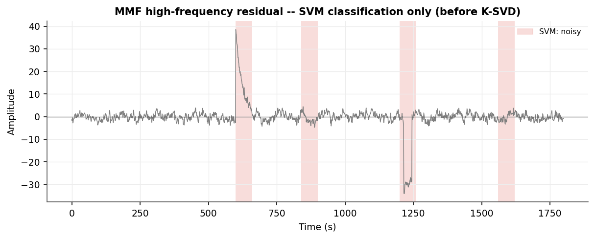
../../_images/tsdenoise_segments_synthetic.png — `plot_ts_denoise_segments()` for the high-frequency residual of the synthetic record introduced in full below. Both genuine transients are shaded, along with two purely random background windows the classifier also flagged – see the false-positive discussion further down for what that costs.#

Note

win_len above (60 samples) is not win_seconds (60 s) – it is win_seconds / dt in samples, the actual embedding length the entropy features see. The paper’s own default, win_seconds=10, is 150 samples at their 15 Hz sampling; at 1 Hz it is only 10 samples, too short for a stable 2-dimensional embedding ((2) needs several dozen points at minimum to estimate reliably) – always check that round(win_seconds / dt) lands in a sane range for the survey’s own sampling rate.

11.27.4.2. Denoising only the flagged windows with K-SVD#

Windows the SVM flags noisy are handed to KSVDDenoiser, which learns a small dictionary directly from overlapping patches of the flagged window itself – no pre-training needed. Given a training-patch matrix \(\mathbf Y\) (one patch per column), dictionary learning via K-SVD [Aharon2006] solves

(3)#\[\min_{\mathbf D,\, \mathbf X} \; \| \mathbf Y - \mathbf D \mathbf X \|_F^2 \quad \text{s.t.} \quad \| \mathbf x_i \|_0 \le s \ \ \forall i,\]

alternating orthogonal matching pursuit (fixing \(\mathbf D\), sparse coding each patch with at most \(s\) active atoms) with a per-atom singular-value update of \(\mathbf D\) – the step that distinguishes K-SVD from a plain alternating-least-squares dictionary fit, and the reason it converges to a better dictionary for a given sparsity budget than earlier methods such as the method of optimal directions. Because a short, low-sparsity dictionary can represent a stereotyped transient far better than the genuinely random background can ever be compressed to, the sparse reconstruction \(\mathbf D\mathbf X\) of a noisy window approximates the noise, not the underlying signal – transform() returns the window minus that reconstruction, and noise_profile() exposes the extracted noise contour on its own. Used directly, rather than through TimeSeriesDenoiser’s per-window calls, on a longer ~4.2-hour real EY segment around the same kap103 burst (long enough that the default n_atoms=64 is not capped down by too few training patches, unlike a single short classification window):

>>> from pycsamt.ai.processing import KSVDDenoiser
>>> low, high = mmf_split(ey_segment, size=241)   # ~3000 samples
>>> den = KSVDDenoiser(random_state=0).fit(high)
>>> den._D.shape[1]      # atoms actually used
64
>>> noise_profile = den.noise_profile(high)
>>> denoised = den.transform(high)
>>> peak = high.argmax()
>>> high[peak], noise_profile[peak], denoised[peak]
(577.14, 577.14, 0.00)

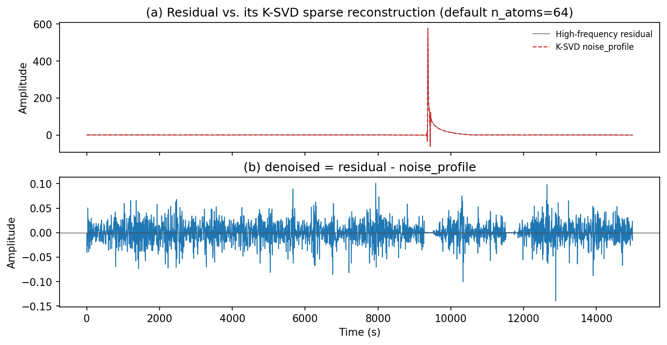
../../_images/tsdenoise_ksvd_direct.png — `KSVDDenoiser` applied directly to the real `EY` segment. (a) the residual and its sparse reconstruction overlap almost everywhere, not just at the peak; (b) what is left after subtracting – small, but visibly structured rather than a flat zero line.#

At the peak, noise_profile matches high almost exactly and denoised is indistinguishable from zero, exactly as intended. Look away from the peak, though, and the same thing is true almost everywhere in this segment: a quiet 300-second stretch with no visible interference at all goes from a raw standard deviation of 0.13 down to 0.02, a 96% reduction, essentially the same reduction the genuine burst gets. With n_atoms=64 and roughly 186 available 32-sample patches in this segment, real long-period natural-field data turns out to be locally smooth enough that a 64-atom dictionary with a sparsity budget of 4 can represent nearly any 32-sample stretch of it well, not only the interference – so KSVDDenoiser behaves less like a surgical noise extractor here and more like an aggressive general sparse-reconstruction smoother. Lowering n_atoms softens this without escaping it:

>>> for n_atoms in (64, 32, 16, 8, 4):
...     d = KSVDDenoiser(n_atoms=n_atoms, random_state=0).fit(high)
...     out = d.transform(high)
...     quiet = out[700:1000]
...     print(n_atoms, d._D.shape[1], round(out.std(), 4), round(quiet.std(), 4))
64 64 0.0203 0.0190
32 32 0.0367 0.0385
16 16 0.0581 0.0652
 8  8 0.0740 0.0912
 4  4 0.5426 0.0991

The quiet-region residual std climbs only from 0.019 to 0.099 – still a 26% reduction on samples with no interference – as n_atoms drops from 64 to 4, while the overall residual std jumps sharply at 4 atoms (0.54, up from 0.07 at 8): too few atoms starts destabilising the SVD update on the genuinely hard-to-represent burst itself rather than protecting the background. There is no n_atoms in this range that both fully preserves quiet-period samples and denoises the burst cleanly for data this smooth – a real trade-off worth knowing about before reading K-SVD’s noise_profile as a clean noise/signal separation on this kind of record, rather than as a strong (and, in aggregate, still net-beneficial) general-purpose local smoother. The fully synthetic record below, whose background is genuinely high-entropy white-ish noise by construction rather than smoothly autocorrelated natural field data, is the case where K-SVD’s intended noise-only behaviour holds much more cleanly – worth keeping in mind when judging which of the two demonstrations below best matches a given survey’s own data character.

11.27.4.3. Validating against a known-clean synthetic record#

No real field recording carries an independent clean twin, so – exactly as Learned Spectral Denoising does for EMDenoiser – the only way to report a genuine before/after number is a synthetic record with a known reference. The one used throughout this section is a 30-minute, 1 Hz channel: a weak, band-limited colored-noise background (1/f^0.6 spectral shape, rescaled to a background standard deviation of 2.0 arbitrary units – the qualitative “weak amplitude, strong randomness” description of a high-quality MT signal), with two transients injected on top: a charge/discharge-like exponential decay (amplitude 40, starting at \(t=600\) s, 25 s decay constant) and a square-wave block (amplitude 30, \(t=1215\)-\(1245\) s).

>>> from pycsamt.ts import TSData
>>> from pycsamt.ai.processing import (
...     TimeSeriesDenoiser, snr_db, time_domain_ncc,
... )
>>> ts = TSData(data={"EX": noisy}, dt=1.0, station="synthetic_demo")
>>> den = TimeSeriesDenoiser(mmf_size=121, win_seconds=60.0, random_state=0)
>>> out = den.apply(ts)
>>> denoised = out.get("EX")
>>> f"{snr_db(clean, noisy):.2f} -> {snr_db(clean, denoised):.2f} dB"
'-6.65 -> 10.25 dB'
>>> f"{time_domain_ncc(clean, noisy):.4f} -> {time_domain_ncc(clean, denoised):.4f}"
'0.3712 -> 0.9519'

A 16.9 dB SNR gain and a normalized cross-correlation climbing from 0.37 to 0.95 both say the same thing: the reconstructed channel is close to the true clean reference, not merely “smoother.” den worked directly on a TSData record via apply() – the same TSData-in/TSData-out convention every other tool in this section follows for site collections – with channels= selecting a subset of channels when only some need denoising and inplace= controlling whether ts itself is mutated. Every window’s classification is recorded on diagnostics_:

>>> diag = den.diagnostics_
>>> diag[diag["label"] == "noisy"]
   channel  win_start  win_stop     score  label
10      EX      600.0     660.0  0.141293  noisy
14      EX      840.0     900.0  0.117761  noisy
20      EX     1200.0    1260.0  0.265015  noisy
26      EX     1560.0    1620.0  0.265149  noisy

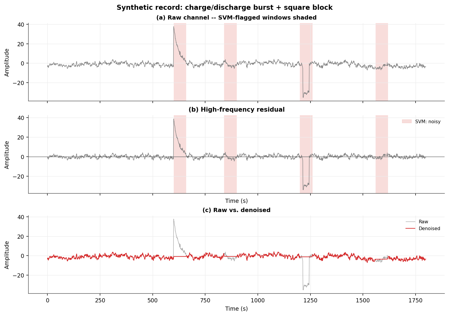
../../_images/tsdenoise_synthetic_summary.png — `plot_ts_denoise_summary()` for the synthetic record. (a) raw channel with SVM-flagged windows shaded; (b) the same shading on the MMF high-frequency residual actually classified; (c) raw vs. denoised.#

Two of the four flagged windows – [600, 660) and [1200, 1260) – contain the two genuine injected transients and are exactly where panel (c) shows the denoised trace collapsing the burst and the square block back toward the background level. The other two, [840, 900) and [1560, 1620), contain no injected interference at all: they are false positives from the SVM, on purely random background that happened to look unusual enough on four features to cross the quality_threshold =0.5 boundary. K-SVD then denoised them anyway, and panel (c) shows the visible cost of that: within [840, 900) the sub-window SNR against the true reference falls from 66.7 dB to 1.7 dB; within [1560, 1620) from 319.0 dB to 7.6 dB. Both windows go from “indistinguishable from the true signal” to “visibly flattened” – a concrete illustration of exactly the failure mode Gui et al. (2024) built the SVM stage to prevent in the first place, occurring here on the roughly 1-in-15 clean windows the classifier still gets wrong. It is a real cost, and worth weighing against the 16.9 dB gained overall: for this record, four windows in thirty being sent to K-SVD – two correctly, two not – was still a large net improvement, but a survey where the signal itself is the primary object of study, rather than a precursor to averaging many stations together, deserves a look at diagnostics_ before trusting an unattended run.

11.27.4.4. Applying the pipeline to a real field recording#

data/MT/TS/kap103as.ts is the bundled SAMTEX/LiMS long-period magnetotelluric recording already used throughout Transformers and the pycsamt.iot edge-QC examples – station kap103, five channels (HX, HY, HZ, EX, EY), 5 s sampling, roughly 27 days, with the small genuine data gaps (under 0.3% of samples) real multi-week field deployments always carry. Its EY channel contains a real burst reaching 582 units against a background comfortably under 10 – read directly with read_ts():

>>> from pycsamt.ts import read_ts, TSData
>>> ts = read_ts("data/MT/TS/kap103as.ts/kap103as.ts")
>>> ts
TSData(station='kap103', chan=[HX,HY,HZ,EX,EY], n=461747, dt=5.0)
>>> ey = ts.get("EY")[341100:341900]   # ~66-minute window around the burst
>>> ey.max()
582.117004

At 5 s sampling, both defaults need overriding for the same reason noted above: win_seconds=10 would be only 2 samples, and the automatic mmf_size would clamp to the minimum 3-sample structuring element – far narrower than this burst’s multi-minute decay tail. Using the tuned mmf_size=241 (1205 s) from the sensitivity sweep earlier and a 300 s classification window:

>>> from pycsamt.ai.processing import TimeSeriesDenoiser
>>> sub = TSData(dt=ts.dt, station=ts.station)
>>> sub.add_channel("EY", ey)
>>> den = TimeSeriesDenoiser(mmf_size=241, win_seconds=300.0, random_state=0)
>>> out = den.apply(sub)
>>> denoised = out.get("EY")
>>> ey.max(), denoised[ey.argmax()]
(582.117004, 4.772685409999772)

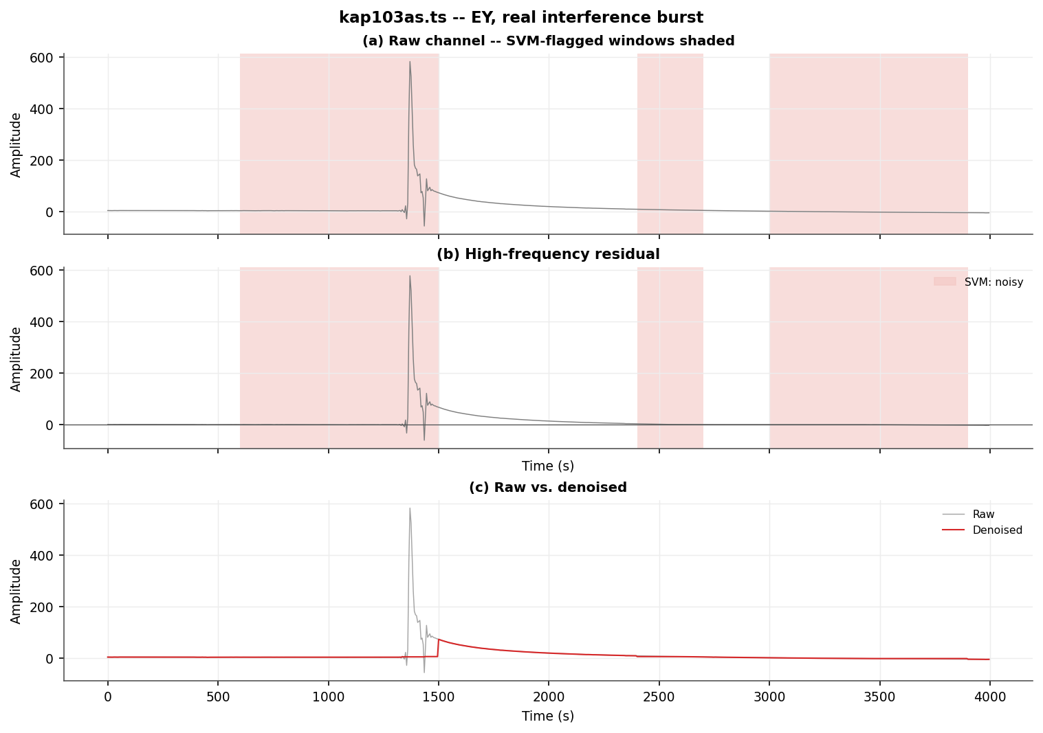
../../_images/tsdenoise_real_summary.png — `plot_ts_denoise_summary()` for the real `kap103as.ts` burst. At this amplitude scale the peak dominates the plot; the three other flagged windows away from it show no visible structure in panel (a), consistent with them being either much smaller genuine anomalies or additional false positives.#

The peak collapses from 582 to 4.8 – close to the channel’s own quiet background – while the slow, minutes-long decay either side of the peak, correctly kept in the low-frequency envelope, is preserved rather than chopped off. Seven of the fourteen 300 s windows in this slice are flagged noisy, not just the one containing the visible peak. Unlike the synthetic case above, there is no independent clean reference here to say how many of the other six are genuine smaller anomalies in a real, imperfect field recording versus additional false positives at roughly the rate quantified above – which is exactly why AI Processing Overview’s closing warning applies here as much as to any other tool in this section: treat diagnostics_ as a prioritisation aid for review, not a silent accept/reject gate.

11.27.4.5. Parameters and limitations#

mmf_size is the single most consequential parameter and, as shown above, unavoidably data-dependent – there is no default that is safe across both a 15 Hz CSAMT survey and 5 s long-period MT. Inspect low (returned by mmf_split(), or via TimeSeriesDenoiser().apply(...)’s internals) against a plot of the raw channel and widen size/mmf_size until any known interference plateau disappears from it.

clean_amp and noise_amp_ratio calibrate the synthetic training library’s amplitude to the channel actually being denoised. Left at an arbitrary fixed scale, every real feature vector would sit far outside the training distribution’s envelope – a regime where a linear SVM’s decision boundary no longer tracks “more extreme means more noisy” and can misclassify confidently rather than uncertainly (Xn far outside the trained range does not reliably extrapolate). Both examples above avoid this because transform(), called automatically from apply() when no classifier is attached yet, derives clean_amp itself from a robust (median-absolute- deviation-based, not plain standard deviation – which the very interference being screened for would inflate) estimate of that channel’s own high-frequency background level, then trains against noise_amp = clean_amp * noise_amp_ratio (default ratio 8.0, matching the roughly 8x contrast Fig. 3 of Gui et al. (2024) shows between their strong-interference and high-quality samples). This self-calibration has its own limit: repeating the synthetic square-wave example above with the block’s amplitude raised from 30 to 35 units (background std still 2.0, so roughly 17.5x rather than 15x) flips its classification outright, from confidently noisy (score 0.265) to barely clean (score 0.535) – a transient genuinely more extreme than roughly twice the trained noise_amp_ratio can end up on the wrong side of a linear boundary fit only within a narrower range. Pass an explicit, larger noise_amp_ratio (or a pre-trained SignalQualityClassifier built the same way) when a survey’s own interference is known to run that extreme.

quality_threshold (default 0.5) is the score boundary between “clean” and “noisy” in diagnostics_; raising it sends fewer windows to K-SVD (fewer false positives like the two illustrated above, at the cost of possibly missing weaker real interference), lowering it does the opposite. patch_len, n_atoms, sparsity, ksvd_iter, and ksvd_overlap control each flagged run’s KSVDDenoiser directly – a larger sparsity budget lets the dictionary represent more complex interference shapes at the risk of also absorbing some genuine signal structure into the “noise” it subtracts.

Note

TimeSeriesDenoiser and SignalQualityClassifier depend on scikit-learn (the linear SVM) and SciPy (grayscale morphology via scipy.ndimage.grey_erosion()/ grey_dilation()); both are already required by other tools in this section and need no extra installation. Unlike EMDenoiser, there is no PyTorch/TensorFlow backend involved – the feature set is small enough that a linear SVM and a dictionary of a few dozen atoms are the appropriate scale of model, not a neural network.

Full signatures: TimeSeriesDenoiser, SignalQualityClassifier, KSVDDenoiser, mmf_split(), compute_entropy_features(), generate_synthetic_library(), snr_db(), time_domain_ncc(), plot_ts_denoise_mmf_split(), plot_ts_denoise_segments(), and plot_ts_denoise_summary(). The lower-level sparse-coding primitives KSVDDenoiser wraps – omp(), omp_batch(), and ksvd_dictionary() – are public for advanced use (a custom patch-extraction or reconstruction scheme) but KSVDDenoiser is the interface every example above uses.

View the complete synthetic-record example sourceClick to inspect and copy the complete code

def run_synthetic_demo(save_dir: Path) -> None:
    print("\n=== TimeSeriesDenoiser -- synthetic record with known ground truth ===")
    t, dt, clean, noisy = make_synthetic_record()

    ts = TSData(data={"EX": noisy}, dt=dt, station="synthetic_demo")
    den = TimeSeriesDenoiser(mmf_size=121, win_seconds=60.0, random_state=0)
    out = den.apply(ts)
    denoised = out.get("EX")
    diag = den.diagnostics_

    n_noisy = int((diag["label"] == "noisy").sum())
    print(f"  {n_noisy}/{len(diag)} windows flagged noisy")
    print(diag.to_string(index=False))

    low, high = mmf_split(noisy, size=121)
    ax = plot_ts_denoise_segments(
        t, high, diag,
        title="MMF high-frequency residual -- SVM classification only "
              "(before K-SVD)",
    )
    _save(ax.figure, save_dir, "tsdenoise_segments_synthetic.png")

    print(f"  SNR  noisy    -> clean ref: {snr_db(clean, noisy):.2f} dB")
    print(f"  SNR  denoised -> clean ref: {snr_db(clean, denoised):.2f} dB")
    print(f"  NCC  noisy    -> clean ref: {time_domain_ncc(clean, noisy):.4f}")
    print(f"  NCC  denoised -> clean ref: {time_domain_ncc(clean, denoised):.4f}")

    # false-positive cost: any flagged window with no injected transient
    injected = np.zeros(len(t), dtype=bool)
    injected[550:750] = True  # generous margin around the decaying burst
    injected[1200:1260] = True
    for _, row in diag[diag["label"] == "noisy"].iterrows():
        lo, hi = int(row["win_start"] / dt), int(row["win_stop"] / dt)
        if not injected[lo:hi].any():
            sub_snr_before = snr_db(clean[lo:hi], noisy[lo:hi])
            sub_snr_after = snr_db(clean[lo:hi], denoised[lo:hi])
            print(
                f"  false-positive window [{row['win_start']:.0f},"
                f" {row['win_stop']:.0f}) s: SNR {sub_snr_before:.1f} ->"
                f" {sub_snr_after:.1f} dB (genuinely clean signal, "
                f"needlessly re-coded)"
            )

    # amplitude at which the square block stops being flagged (see
    # "Parameters and limitations")
    for amp in (30.0, 35.0):
        noise = np.zeros(len(t))
        env = 40.0 * np.exp(-np.maximum(t - 600.0, 0.0) / 25.0)
        env[t < 600.0] = 0.0
        noise += env
        noise[1215:1245] -= amp
        ts_amp = TSData(data={"EX": clean + noise}, dt=dt, station="amp_sweep")
        den_amp = TimeSeriesDenoiser(mmf_size=121, win_seconds=60.0, random_state=0)
        den_amp.apply(ts_amp)
        hit = den_amp.diagnostics_
        hit = hit[(hit["win_start"] <= 1230) & (1230 < hit["win_stop"])]
        print(
            f"  square amplitude {amp:.0f} (background std ~2): window "
            f"label={hit['label'].values[0]!r} score={hit['score'].values[0]:.3f}"
        )

    fig = plot_ts_denoise_summary(
        t, noisy, denoised, diag, low=low, high=high,
        suptitle="Synthetic record: charge/discharge burst + square block",
    )
    _save(fig, save_dir, "tsdenoise_synthetic_summary.png")

Point read_ts(...) at your own field .ts/.asc file to adapt this script