
12.3. The Airborne Site View#
AirborneSite and
AirborneSites give a flat,
Sites-shaped view over AirborneEMLine/
AirborneEMDataset records – one wrapped
AirborneEMRecord per sample, read directly
from its EMTF document. Unlike
Site, whose numeric accessors all route
through a materialized EDI, an AirborneSite
has no EDI bridge and no impedance requirement, so it can hold a
tipper, an interstation transfer function, a scalar tilt reading, or
a MobileMT admittance tensor equally, and read whichever one its
EMTF document actually carries. This page works entirely from the
four sample surveys committed under data/AFMAG/, data/ZTEM/,
and data/mobileMT/ – see Airborne Data Model Overview for what each represents
– rather than the small hand-built lines Flight Lines and Datasets constructs
from scratch.
12.3.1. Reading Sample Surveys#
ensure_asites() is the single entry point
every airborne-aware emtools function coerces its input through,
and it reads a directory of EMTF-XML files directly into an
AirborneSites:
>>> from pycsamt.airborne.site import ensure_asites
>>> ztem = ensure_asites("data/ZTEM/gold_springs_nv")
>>> len(ztem), ztem.technologies
(105, ('ztem',))
>>> afmag_o = ensure_asites("data/AFMAG/abitibi_on")
>>> len(afmag_o), afmag_o.technologies
(13, ('afmag_original',))
>>> afmag_a = ensure_asites("data/AFMAG/yulong_belt_cn")
>>> len(afmag_a), afmag_a.technologies
(11, ('afmag_airmt',))
>>> mmt = ensure_asites("data/mobileMT/flammefjeld_greenland")
>>> len(mmt), mmt.technologies
(12, ('mobilemt',))
Four different directories, four different AFMAG-family or
ZTEM/MobileMT deliveries, and the same one-line call reads all of
them. technologies is not
supplied by the caller anywhere above – each
AirborneSite resolves its own
technology from the
underlying EMTF.subtype, written by whichever build_*_line
constructor produced the document in the first place (ztem,
mobilemt, afmag_original, or afmag_airmt – the two AFMAG
generations are kept as genuinely distinct labels, not folded into one
"afmag" tag, since their response shapes below are not
interchangeable).
12.3.2. Four Response Families#
has_component() checks
which of those response shapes a given site actually carries, without
having to inspect EMTF.subtype by hand:
>>> afmag_o_site = afmag_o[0]
>>> afmag_a_site = afmag_a[4]
>>> ztem_site = ztem.get("GO_L4_008")
>>> mmt_site = mmt[0]
>>> for s in (afmag_o_site, afmag_a_site, ztem_site, mmt_site):
...     print(
...         s.name, s.technology,
...         "tipper=", s.has_component("tipper"),
...         "interstation_tensor=", s.has_component("interstation_tensor"),
...         "afmag_tilt=", s.has_component("afmag_tilt"),
...         "admittance=", s.has_component("admittance"),
...     )
AB_001 afmag_original tipper= False interstation_tensor= False afmag_tilt= True admittance= False
YU_005 afmag_airmt tipper= False interstation_tensor= True afmag_tilt= False admittance= False
GO_L4_008 ztem tipper= True interstation_tensor= False afmag_tilt= False admittance= False
FL_001 mobilemt tipper= False interstation_tensor= False afmag_tilt= False admittance= True
Each site carries exactly one of the four – a diagonal, not a
coincidence: AirborneSite never fabricates a component a
technology does not measure, so afmag_tilt_deg stays None on
a ZTEM site and tipper stays None on a MobileMT site, rather
than either silently returning zeros. Plotting all four against
frequency, on their own natural axes, makes the physical difference
concrete:
>>> import numpy as np
>>> import matplotlib.pyplot as plt
>>> def frobenius(arr):
...     axes = tuple(range(1, arr.ndim))
...     return np.sqrt(np.sum(np.abs(arr) ** 2, axis=axes))
>>> fig, axes = plt.subplots(2, 2, figsize=(10.0, 7.2))
>>> ax = axes[0, 0]
>>> _ = ax.plot(afmag_o_site.freq, afmag_o_site.afmag_tilt_deg, "o", ms=8, color="C0")
>>> _ = ax.axhline(0.0, color="0.6", lw=0.8)
>>> _ = ax.set_title(f"afmag_original -- {afmag_o_site.name}")
>>> _ = ax.set_xlabel("Frequency [Hz]"); _ = ax.set_ylabel("Tilt angle [deg]")
>>> ax = axes[0, 1]
>>> mag = frobenius(afmag_a_site.interstation_tensor)
>>> _ = ax.semilogx(afmag_a_site.freq, mag, "o-", color="C1")
>>> _ = ax.set_title(f"afmag_airmt -- {afmag_a_site.name}")
>>> _ = ax.set_xlabel("Frequency [Hz]"); _ = ax.set_ylabel(r"$\|\mathbf{T}\|_F$ (interstation tensor)")
>>> ax = axes[1, 0]
>>> mag = frobenius(ztem_site.tipper)
>>> _ = ax.plot(ztem_site.freq, mag, "o-", color="C2")
>>> _ = ax.set_title(f"ztem -- {ztem_site.name}")
>>> _ = ax.set_xlabel("Frequency [Hz]"); _ = ax.set_ylabel(r"$\|\mathbf{T}\|_F$ (tipper)")
>>> ax = axes[1, 1]
>>> mag = frobenius(mmt_site.admittance)
>>> _ = ax.loglog(mmt_site.freq, mag, "o-", color="C3")
>>> _ = ax.set_title(f"mobilemt -- {mmt_site.name}")
>>> _ = ax.set_xlabel("Frequency [Hz]"); _ = ax.set_ylabel(r"$\|\mathbf{Y}\|_F$ (admittance)")
>>> fig.tight_layout()
>>> fig.savefig("user-guide-airborne-site-01.png", dpi=200, bbox_inches="tight")
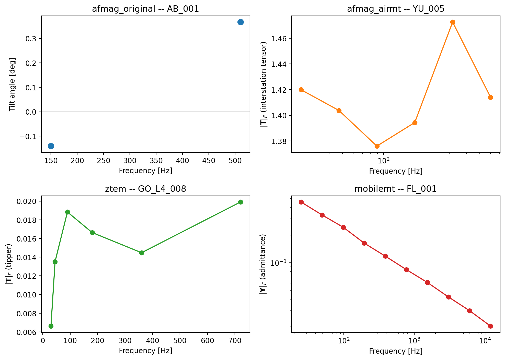
The four response families read from one common container, each on its own natural axis.#
The historical comparator (top left) samples only two audio-frequency
bands, 150 and 510 Hz, and reports a signed tilt in degrees
– station AB_001 reads slightly negative at 150 Hz and
positive at 510 Hz, a genuine sign reversal between bands rather
than measurement noise, since the comparator has no
polarization-ellipse decomposition to average over. AirMt’s
interstation tensor (top right) and ZTEM’s tipper (bottom left) are
both plotted as a per-frequency Frobenius norm across every
component, since neither reduces naturally to one scalar component
the way the comparator’s tilt does; MobileMT’s admittance
(bottom right) is shown on log-log axes because it falls off by more
than an order of magnitude across its ten-decade frequency range,
\(H = Y E\) weakening steadily as frequency rises exactly as
Airborne Natural-Source EM: AFMAG, ZTEM, And MobileMT derives for a fixed source-receiver geometry.
12.3.3. Selecting And Grouping#
AirborneSites indexes by position or
by case-insensitive name, and select()
filters by an explicit name list or a predicate:
>>> ztem[0]
AirborneSite(name='GO_L1_001', technology='ztem', nfreq=6, coords=(37.98404,-114.15000,1750.0))
>>> ztem["GO_L1_001"] is ztem.get("GO_L1_001")
True
>>> line4 = ztem.select(predicate=lambda s: s.name.split("_")[1] == "L4")
>>> len(line4), line4[0].name, line4[-1].name
(15, 'GO_L4_001', 'GO_L4_015')
gold_springs_nv’s station names encode a flight-line label
directly (GO_L<n>_<seq>), so grouping by line here is a one-line
predicate over name.
line_ids is not an
alternative way to reach the same grouping, though:
>>> ztem.line_ids
()
Reading straight from a directory via
from_xml_dir() (what
ensure_asites does above) constructs every site with
line_id=None – the file itself carries no flight-line identifier,
only the station name does by convention. line_id is populated
only when sites are built from an already-assembled
AirborneEMLine, via
from_line():
>>> from pycsamt.airborne import NavigationTrack
>>> from pycsamt.airborne.ztem import build_ztem_line, ZTEMSystemSpec
>>> from pycsamt.airborne.site import AirborneSites
>>> nav = NavigationTrack(
...     sample_ids=("S00", "S01"),
...     easting=np.array([0.0, 50.0]),
...     northing=np.array([0.0, 0.0]),
... )
>>> tip = np.zeros((2, 1, 2), dtype=complex)
>>> tip[:, 0, 0] = [0.01 + 0.002j, 0.015 + 0.001j]
>>> tip[:, 0, 1] = [0.003 - 0.001j, 0.004 - 0.0005j]
>>> line = build_ztem_line(
...     "DEMO", nav, tip, frequency=np.array([90.0]),
...     system_spec=ZTEMSystemSpec(),
... )
>>> AirborneSites.from_line(line).line_ids
('DEMO',)
The distinction matters because ensure_asites is the entry point
every airborne emtools function actually receives – so any code
that groups stations by line_id rather than through the document’s
own metadata will silently see nothing on data read from a directory.
ZTEM Total-Divergence, Phase-Rotation, And Map-View Diagnostics avoids exactly this trap by reading the flight-line
label back out of EMTF.metadata["notes"]["ZTEM"]["LineId"] instead
of relying on line_id; the station-name predicate used above is a
second, equally valid way to reach the same grouping when the survey’s
naming convention already encodes it.
closest() finds the nearest
site to a target coordinate by great-circle distance, with an optional
distance cutoff:
>>> nearest = ztem.closest(37.979, -114.1455)
>>> nearest.name
'GO_L5_009'
>>> ztem.closest(37.979, -114.1455, tol=60.0).name
'GO_L5_009'
>>> ztem.closest(37.979, -114.1455, tol=30.0) is None
True
GO_L5_009 sits about 39 m from the target coordinate – inside a
60 m tolerance, outside a 30 m one, so the same query returns the
station or None depending on how far away “close enough” is
allowed to be.
Note
AirborneSites deliberately does not mirror every
Sites bulk-editing method. There is no edit_all,
with_topography, or to_profile here – those are real
Sites features this module does not yet need for the
emtools integration it exists to unblock, left out rather than
stubbed with placeholder behaviour.
12.3.4. One Container, Three Diagnostics#
The point of reading every technology through the same
AirborneSites container is not just
tidy code – it is that the container needs no conversion to reach
each technology’s own, literature-derived diagnostic. ztem,
afmag_o, and mmt above are handed directly to
plot_ztem_map(),
plot_original_afmag_dual_frequency_profile(),
and plot_mobilemt_conductivity_psection()
– each built around a specific literature source (Legault et al.
2012’s map-view grid, Ward (1959) Fig. 16’s dual-frequency profile,
and the theoretical admittance-to-conductivity relationship Prikhodko
et al. (2022) describe for MobileMT), none of which take anything
other than an AirborneSites-like object as their first argument:
>>> from pycsamt.emtools.ztem import plot_ztem_map
>>> from pycsamt.emtools.afmag import plot_original_afmag_dual_frequency_profile
>>> from pycsamt.emtools.mobilemt import plot_mobilemt_conductivity_psection
>>> fig, (ax1, ax2, ax3) = plt.subplots(1, 3, figsize=(16.5, 5.6))
>>> _ = plot_ztem_map(ztem, ax=ax1)
>>> _ = plot_original_afmag_dual_frequency_profile(afmag_o, ax=ax2)
>>> _ = plot_mobilemt_conductivity_psection(mmt, ax=ax3)
>>> for ax in (ax1, ax2, ax3):
...     ax.title.set_fontsize(10)
>>> fig.tight_layout(w_pad=2.5)
>>> fig.savefig("user-guide-airborne-site-02.png", dpi=200, bbox_inches="tight")
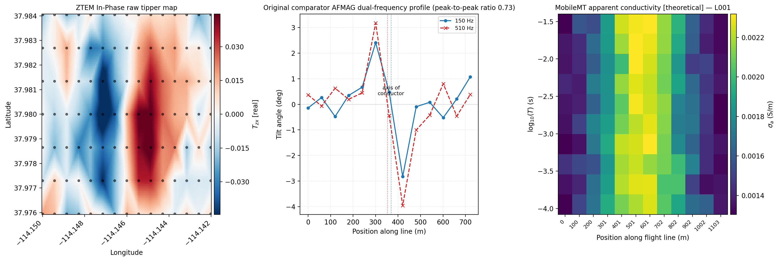
Three technologies, three EMTF-XML directories, three real diagnostics – none of them written for this page.#
Each panel is genuinely reading its own physics. The ZTEM map (left)
grids the in-phase \(T_{zx}\) across all seven gold_springs_nv
lines and finds the same synthetic conductor this page’s earlier
figures already touched: a blue-to-red crossover striking
north-south, strongest through the survey’s centre where the target’s
along-strike amplitude peaks. The AFMAG profile (middle) reproduces
Ward’s own reading of a comparator survey – both frequencies swing
through zero together near station distance 360 m, “the axis of
conductor” the annotation marks, and their differing peak-to-peak
amplitudes (the panel’s title reports the ratio) are exactly the
frequency-dependence Ward used to argue for a real conductor rather
than topographic noise. The MobileMT pseudosection (right) images
theoretical apparent conductivity against period and along-line
position: the brighter band sitting under roughly 400-700 m is
the same kind of central-line response the ZTEM map shows spatially,
here resolved with period as a rough proxy for depth instead of a
second horizontal axis. Interpreting any one of these three panels in
depth is exactly what ZTEM Total-Divergence, Phase-Rotation, And Map-View Diagnostics, AFMAG Tilt-Angle Diagnostics And Motion-Coupling Physics, and
MobileMT Admittance, Apparent Conductivity, And Skew Diagnostics are for; this page’s point is narrower –
every panel above started from nothing more than a directory path and
ensure_asites().
12.3.5. Exporting And Round-Tripping#
to_dataframe() exports one
site’s data to a tidy, frequency-indexed table:
>>> ztem_site.to_dataframe(kind="tipper").round(4)
                   Tx              Ty
f
30.0  -0.0012-0.0038j -0.0004-0.0052j
45.0  -0.0041+0.0059j -0.0084+0.0078j
90.0   0.0145-0.0024j -0.0079-0.0087j
180.0  0.0075+0.0116j  0.0091-0.0018j
360.0 -0.0070-0.0078j -0.0046-0.0088j
720.0  0.0092-0.0163j  0.0052-0.0045j
and write_xml() writes an
entire collection back out, one EMTF-XML file per site, which
from_xml_dir() can read
straight back in – a genuine round trip through the file format, not
just an in-memory copy:
>>> import tempfile
>>> with tempfile.TemporaryDirectory() as tmp:
...     paths = afmag_a.write_xml(tmp)
...     reread = AirborneSites.from_xml_dir(tmp)
...     orig = afmag_a.get("YU_005")
...     back = reread.get("YU_005")
...     tensors_match = np.allclose(orig.interstation_tensor, back.interstation_tensor)
...     freqs_match = np.allclose(orig.freq, back.freq)
>>> len(paths), len(reread)
(11, 11)
>>> tensors_match, freqs_match
(True, True)
The interstation tensor and frequency grid both survive the
write-then-read cycle exactly, confirming that
to_xml() – called once per
site under write_xml – serializes the full (n_f, 3, 2) array
rather than truncating it to the (n_f, 1, 2) shape a tipper-only
document would need.