11.14. AFMAG Tilt-Angle Diagnostics And Motion-Coupling Physics#

AFMAG (audio-frequency magnetics) is a passive electromagnetic method with no electric-field channel [Ward1959]. Where a full MT survey records the horizontal electric and magnetic fields to build an impedance tensor, AFMAG systems – whether the historical two-coil comparator or a modern tensor system such as ZTEM/AirMt – work from magnetic-field components alone. The historical readout is a scalar “tilt angle” describing how far the resultant magnetic-field polarization ellipse departs from horizontal; the modern readout is a full interstation magnetic transfer function. Both are, in the transfer-function language pyCSAMT already uses everywhere else, the same object as the tipper,

\[H_z(f) = T_x(f)\,H_x(f) + T_y(f)\,H_y(f),\]

with \(T_x\) and \(T_y\) the complex, frequency-dependent tipper components. pycsamt.emtools.afmag is therefore built entirely on Site.tipper, the same array every other tipper tool in pycsamt.emtools reads – see Transfer Functions And Tipper Diagnostics – and never touches Site.z.

This page covers three genuinely different pieces of work that share one module:

Piece	Main tools	Purpose
Tilt-angle diagnostics	`afmag_tilt_angles`, `plot_afmag_tilt_profile`, `plot_afmag_tilt_psection`, `plot_afmag_tilt_polar`	Read a classical AFMAG tilt angle out of already-assembled tipper data (demonstrated below on a real ground MT tipper, reused for its geometry).
Motion-coupling physics and QC	`euler_rotation_matrix`, `motion_coupling_cosine`, `motion_susceptibility_table`, `flag_motion_susceptible_band`	Simulate and flag the platform-attitude noise described by [Liu2018], using raw attitude and geomagnetic geometry rather than tipper data.
AFMAG-family diagnostics on real airborne data	`original_afmag_tilt_table`, `original_afmag_conductor_diagnostics`, `airmt_tilt_angles`, `plot_airmt_tilt_psection`, `compute_airmt_amplification_parameter`	Read the two real, genuinely different AFMAG-family response shapes (Section Two Response Families, On Real Airborne Data below) from `AirborneSites`, on two committed synthetic airborne surveys.

All public functions used below are exported from pycsamt.emtools (the first two pieces) or from pycsamt.emtools.afmag directly (the third).

11.14.1. Use A Dataset With Tipper#

No AFMAG vendor has supplied pyCSAMT with a real field delivery (see the project’s airborne-EM roadmap for that decision), so data/AFMAG/ carries synthetic sample surveys rather than a real one – Two Response Families, On Real Airborne Data below reads those directly. Before that, this section and the two after it instead reuse the bundled KAP03 long-period MT profile, the same 26-station survey used throughout Transfer Functions And Tipper Diagnostics, purely as a source of a genuine complex (Tx, Ty) tipper. KAP03 is a ground MT survey, not an airborne AFMAG survey – it is reused here only because AFMAG’s tilt angle and the MT tipper are mathematically the same quantity, so KAP03’s real tipper is a legitimate, reproducible input for exercising the tilt-angle transformation on a large, genuinely real dataset before moving to the smaller synthetic airborne surveys. Nothing about attitude, altitude, or flight geometry in the figures below is real; that part is demonstrated separately, below, with an explicitly synthetic attitude time series.

>>> from pathlib import Path
>>> from pycsamt.emtools import ensure_sites
>>> edi_dir = Path("data/MT/kap03lmt_edis")
>>> sites = ensure_sites(edi_dir, recursive=True, strict=False)
>>> print(len(sites), "stations")
26 stations

11.14.2. What The Tilt Angle Represents#

Ward’s original AFMAG comparator reported an in-phase and a quadrature tilt reading from two crossed receiver coils [Ward1959]. In tipper terms, treating the resultant horizontal-to-vertical ratio as a small angle,

\[\theta_\mathrm{tilt}(f) = \arctan\bigl|\mathbf{T}_c(f)\bigr|, \qquad \bigl|\mathbf{T}_c(f)\bigr| = \sqrt{T_{x,c}(f)^2 + T_{y,c}(f)^2},\]

where \(c\) selects the real (in-phase), imaginary (quadrature), or complex-magnitude component of the tipper – exactly the same component split Transfer Functions And Tipper Diagnostics uses for induction arrows. Using \(\arctan\) rather than the ratio itself keeps the reported angle bounded as \(|\mathbf{T}_c|\) grows, and reduces to the classical small-angle reading (\(\theta \approx |\mathbf{T}_c|\) in radians) whenever the ratio is genuinely small, which is the normal case. afmag_tilt_angles returns this quantity, in degrees, for every station and frequency, as a tidy table – the same sites-in/DataFrame-out shape as psd_table() and coherence_table():

>>> from pycsamt.emtools import afmag_tilt_angles
>>> table = afmag_tilt_angles(sites)
>>> table.shape
(518, 8)
>>> list(table.columns)
['station', 'freq', 'period', 'tilt_real_deg', 'tilt_real_azimuth_deg', 'tilt_imag_deg', 'tilt_imag_azimuth_deg', 'tilt_resultant_deg']

Each row is one station-frequency sample. tilt_real_deg and tilt_imag_deg are the in-phase and quadrature readings; the _azimuth_deg columns record the same real/imaginary induction-arrow direction Transfer Functions And Tipper Diagnostics already plots, now labelled for AFMAG’s amplitude reading rather than a map direction; tilt_resultant_deg folds real and imaginary magnitude together, \(\arctan\sqrt{|T_x|^2+|T_y|^2}\), and is the best single column for “how anomalous is this station”, independent of phase.

11.14.3. Tilt-Angle Profile#

The classic AFMAG field product is a profile of tilt angle along one flight line. plot_afmag_tilt_profile reproduces that view for a Sites collection, at one reference period:

>>> from pycsamt.emtools import plot_afmag_tilt_profile
>>> ax = plot_afmag_tilt_profile(sites, component="real", period_s=650.0)
>>> ax.figure.savefig("afmag_tilt_profile.png", dpi=200, bbox_inches="tight")

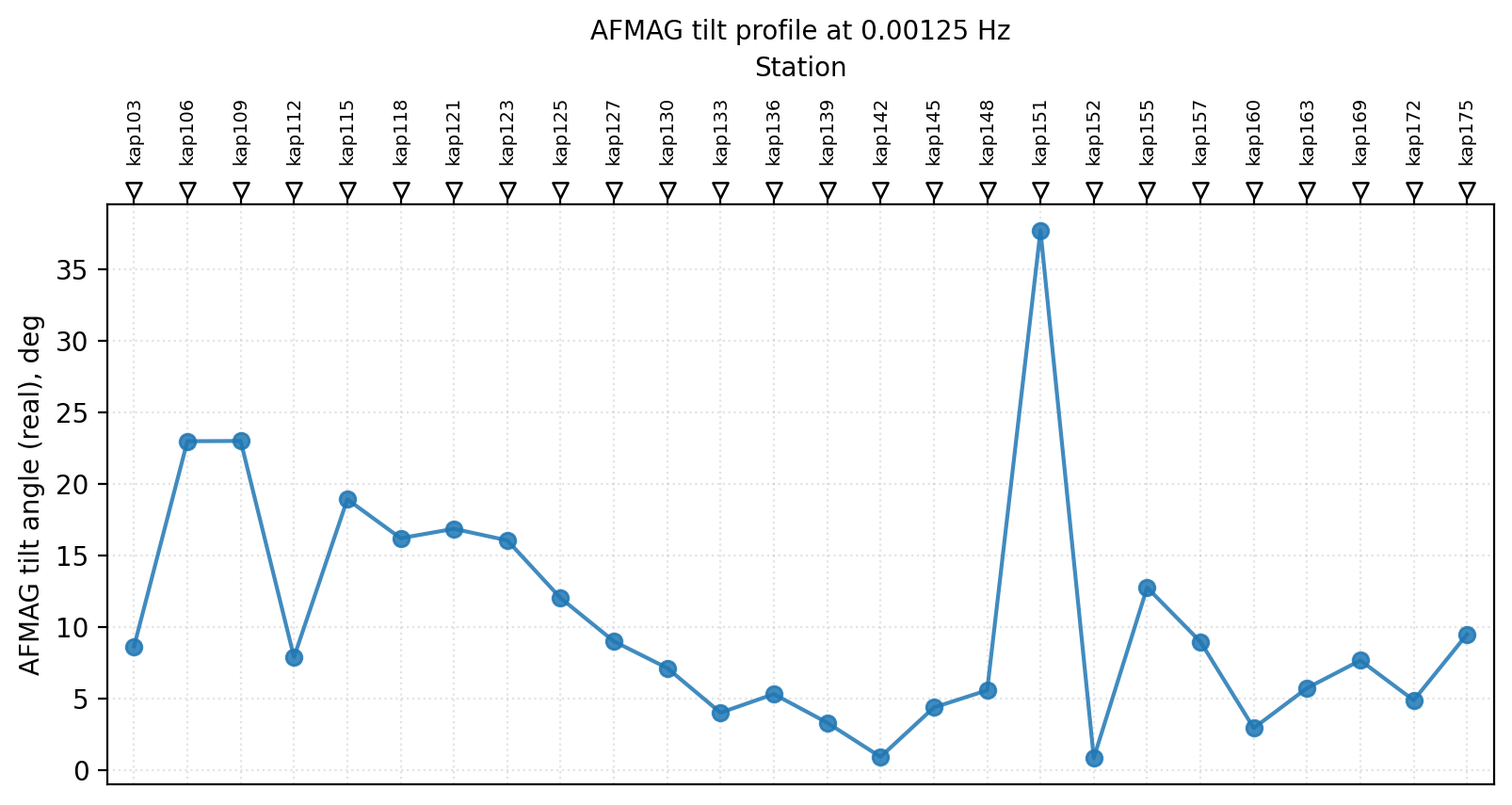
One station stands out immediately: kap151 reaches roughly \(38^\circ\), well over four times the survey median, while its neighbours kap148 and kap152 sit near \(5^\circ\)-6\(^\circ\).

>>> sub = table[table["station"] == "kap151"]
>>> row = sub.iloc[(sub["freq"] - 1 / 650.0).abs().argmin()]
>>> print("kap151 tilt (real):", round(row["tilt_real_deg"], 1), "deg at", row["period"], "s")
kap151 tilt (real): 37.7 deg at 800.0 s
>>> sub2 = table[table["station"] == "kap103"]
>>> row2 = sub2.iloc[(sub2["freq"] - 1 / 650.0).abs().argmin()]
>>> print("kap103 tilt (real):", round(row2["tilt_real_deg"], 1), "deg")
kap103 tilt (real): 8.6 deg

This is not a coincidental pick: kap151 is the same station flagged independently on Transfer Functions And Tipper Diagnostics, where its Tx hodogram traces a large, coherent loop reaching well outside the unit circle. A single AFMAG tilt profile and a full-tensor tipper hodogram are answering related but different questions – amplitude-only versus complex-plane shape – and here they agree: this is a genuinely strong, coherent response, not scatter that happens to average to a large angle.

11.14.4. Tilt-Angle Pseudosection#

A profile at one period hides how the anomaly evolves with depth. plot_afmag_tilt_psection images the resultant tilt over station and log-period at once, the same station-x-period layout plot_induction_section() already uses for the tipper:

>>> from pycsamt.emtools import plot_afmag_tilt_psection
>>> ax = plot_afmag_tilt_psection(sites, component="resultant")
>>> ax.figure.savefig("afmag_tilt_psection.png", dpi=200, bbox_inches="tight")

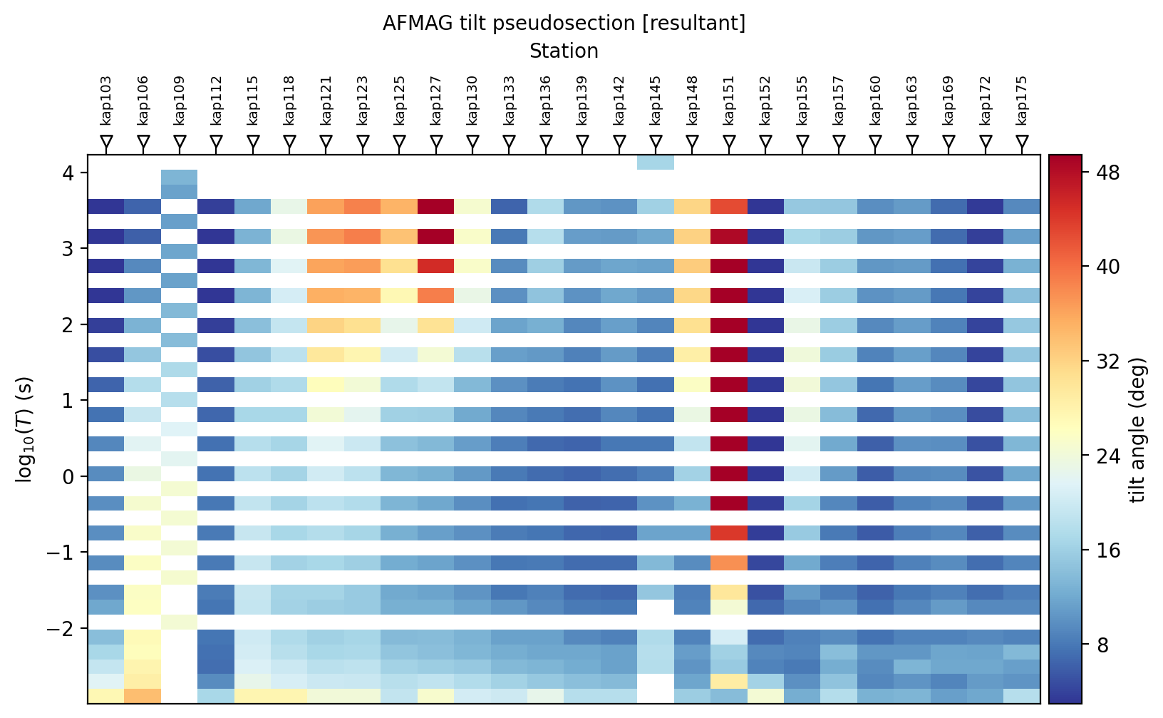
../../_images/user-guide-emtools-afmag-02.png

kap151 is again the standout, but the section adds information the single-period profile could not: its elevated tilt persists across almost the entire sampled period range, not just at \(650\) seconds, and a second, weaker cluster (kap121-kap127) is elevated mainly at short-to-mid period. A station that stays anomalous from the shortest to the longest period sampled – as kap151 does here – points to a different kind of feature than one that is only strong in a narrow window, and is worth a closer, station-level look before drawing conclusions from the profile alone.

11.14.5. Single-Station Tilt Polar View#

plot_afmag_tilt_polar is the AFMAG-labelled counterpart of plot_tipper_polar(): one scatter point per frequency, radius is the \(\arctan\)-tilt magnitude, angle is the induction-arrow azimuth, colour is \(\log_{10}(\text{period})\).

>>> from pycsamt.emtools import plot_afmag_tilt_polar
>>> ax = plot_afmag_tilt_polar(sites, station="kap151", component="real")
>>> ax.figure.savefig("afmag_tilt_polar.png", dpi=200, bbox_inches="tight")

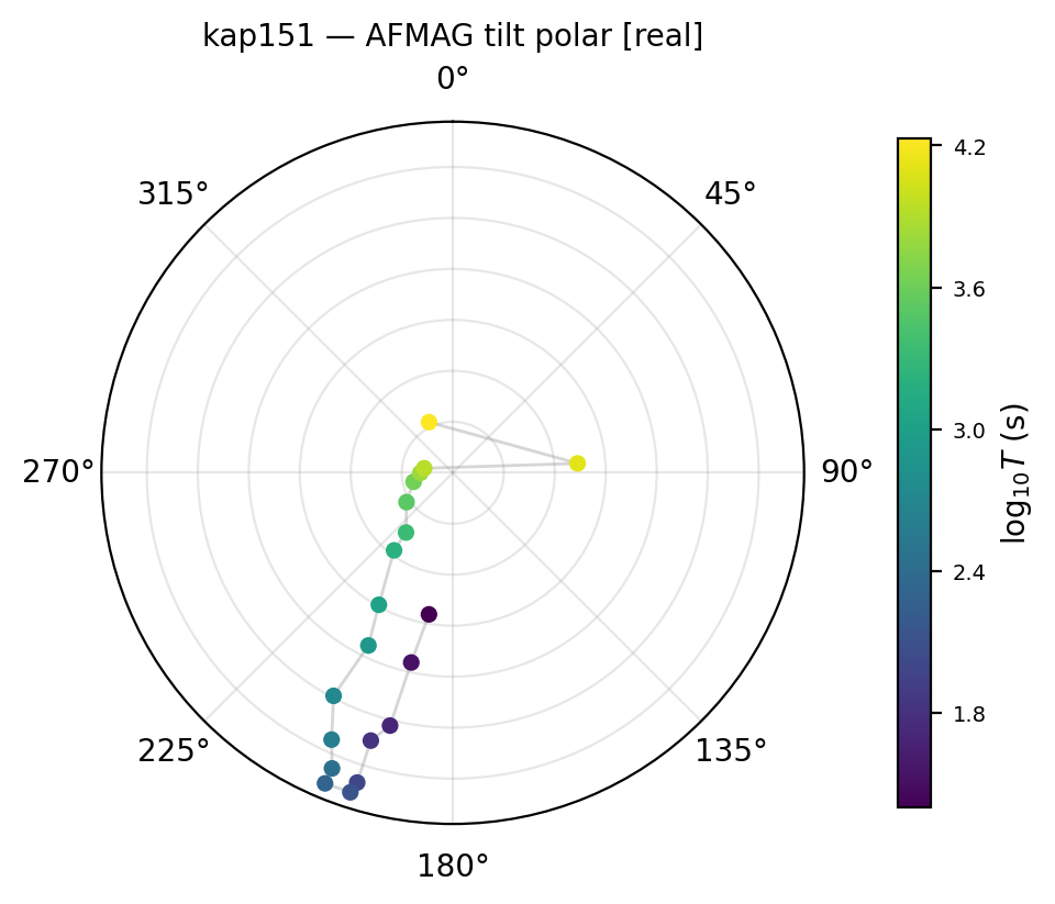
../../_images/user-guide-emtools-afmag-03.png

The points trace a coherent path from short period (dark, near \(180^\circ\)-\(225^\circ\)) through mid period and back toward long period (bright yellow, near \(90^\circ\)) rather than scattering randomly across the disk. A smooth path like this is the polar-view equivalent of the coherent hodogram loop noted on Transfer Functions And Tipper Diagnostics: evidence that kap151’s response evolves systematically with period, which is exactly what should make a single-period profile value like the \(38^\circ\) reading above trustworthy rather than a one-off outlier.

11.14.6. Motion-Induced Noise: The Rotation-Matrix Method#

Airborne AFMAG data are collected on a moving platform, and the receiver coil’s own attitude changes constantly relative to the local geomagnetic field. That changing attitude alone – with no subsurface signal involved at all – induces a voltage in the coil, because the magnetic flux through it changes as the coil tilts. This motion-induced noise can be one to two orders of magnitude larger than the natural-source signal at low frequency, which is exactly the frequency range AFMAG depends on [Liu2018].

Liu et al. (2018) introduce a rotation-matrix method to simulate this noise directly from the coil’s measured attitude, so it can be subtracted from the raw signal. Two Cartesian frames are involved: a fixed local frame \(L\) (east, north, up) and a frame \(S\) attached to the coil, which coincide when the coil is level. A standard aerospace “airline convention” Tait-Bryan rotation – yaw \(\psi\) about \(Z_S\), then pitch \(\theta\) about the once-rotated \(Y_S'\), then roll \(\phi\) about the twice-rotated \(X_S''\) – carries a vector from \(S\) into \(L\):

\[R_{LS}(\psi,\theta,\phi) = R_z(\psi)\,R_y(\theta)\,R_x(\phi).\]

euler_rotation_matrix builds \(R_{LS}\) directly from this definition. It is a genuine rotation for any input angle – orthogonal with determinant \(+1\) – and reduces to the identity at zero attitude:

>>> from pycsamt.emtools import euler_rotation_matrix
>>> import numpy as np
>>> R = euler_rotation_matrix(0.0, 0.0, 0.0)
>>> np.round(R, 6)
array([[ 1.,  0.,  0.],
       [ 0.,  1.,  0.],
       [-0.,  0.,  1.]])

For a single z-axis coil, the sensor’s own normal is \(N_S=(0,0,1)^T\), so its direction in the fixed frame is simply the third column of \(R_{LS}\), computed by coil_normal_direction. The local geomagnetic field direction follows from its inclination \(I\) (dip below horizontal, positive downward) and declination \(D\) (bearing from geographic north toward east),

\[\hat{B}_E = \bigl(\cos I \sin D,\ \cos I \cos D,\ -\sin I\bigr),\]

built by geomagnetic_field_direction. KAP03 sits at roughly \(-22^\circ\) to \(-32^\circ\) latitude (southern Africa); \(I=-62^\circ\), \(D=-20^\circ\) below are representative round values for that region, not an IGRF lookup for a specific station and epoch – for real survey work, obtain the true local inclination/declination from a proper geomagnetic reference model instead.

>>> from pycsamt.emtools import geomagnetic_field_direction
>>> b = geomagnetic_field_direction(-62.0, -20.0)
>>> np.round(b, 4)
array([-0.1606,  0.4412,  0.8829])

The negative inclination correctly points the field mostly upward (the positive “up” component), matching the real Southern-Hemisphere sense of the geomagnetic field. The angle between the field and the coil normal, and its cosine, are the quantities that actually drive the noise:

\[\cos\theta(t) = \hat{B}_E \cdot N_L(t), \qquad V(t) \propto -\,\frac{d\bigl(\cos\theta(t)\bigr)}{dt},\]

computed by motion_coupling_cosine/motion_coupling_angle and simulate_motion_induced_voltage respectively.

Liu et al. (2018) characterize this coupling before ever touching real data, by sweeping \(\theta(t)\) and \(\cos\theta(t)\) over roll, pitch, and yaw at several inclinations, at zero declination (their Fig. 2). That sweep is itself synthetic – it is testing the model, not measuring anything – so it is entirely reproducible from the functions above with no time series at all:

>>> import matplotlib.pyplot as plt
>>> from pycsamt.emtools import motion_coupling_angle
>>> angles = np.linspace(-90.0, 90.0, 181)
>>> zeros = np.zeros_like(angles)
>>> fig, axes = plt.subplots(2, 3, figsize=(12.0, 6.5), sharex="col", sharey="row")
>>> for inc in (-30.0, -50.0, -70.0, -90.0):
...     theta_roll = motion_coupling_angle(zeros, zeros, angles, inc, 0.0)
...     theta_pitch = motion_coupling_angle(zeros, angles, zeros, inc, 0.0)
...     theta_yaw = motion_coupling_angle(angles, zeros, zeros, inc, 0.0)
...     _ = axes[0, 0].plot(angles, theta_roll, label=f"I={inc:g}°")
...     _ = axes[0, 1].plot(angles, theta_pitch)
...     _ = axes[0, 2].plot(angles, theta_yaw)
>>> print("yaw-sweep theta is constant at I=-90:", theta_yaw.std() < 1e-9)
yaw-sweep theta is constant at I=-90: True

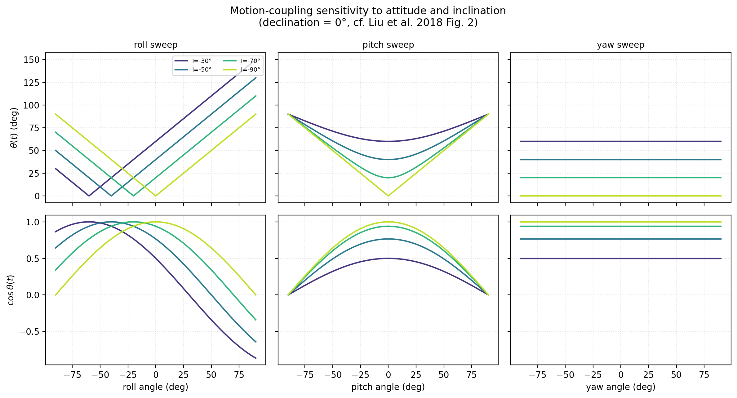
../../_images/user-guide-emtools-afmag-04.png

Three behaviours match Liu et al. (2018)’s own description exactly. Roll (left column): \(\theta(t)\) is piecewise linear in roll, and changing inclination shifts the V-shaped curve sideways without changing its slope – the paper’s own “sharp turns of the curve… decided by the definition of Eq. 7” for the acute-angle bound. Pitch (middle column): the curves are smoothly concave, and inclination sets the floor value at zero pitch – both amplitude and shape now depend on inclination, because pitch’s rotation axis is not perpendicular to the coil plane the way roll’s and yaw’s are. Yaw (right column): every curve is perfectly flat – yaw has no effect on \(\theta(t)\) at zero pitch/roll, confirmed numerically above, and only the inclination sets each line’s height. This is the same zero-yaw-sensitivity property the module’s own test suite checks for a z-axis coil, because a yaw rotation is a rotation about the coil’s own normal, which cannot change the angle between that normal and anything else.

With the model itself characterized, one illustrative attitude segment shows what a single short flight interval looks like in practice – an explicit random seed, no real INS data is bundled with pyCSAMT – with a slow platform oscillation at the small-angle amplitudes Liu et al. (2018) themselves used for their own literature comparison (“angular range of 10 degrees”):

>>> from pycsamt.emtools import plot_motion_coupling
>>> rng = np.random.default_rng(42)
>>> t = np.linspace(0.0, 20.0, 400)
>>> yaw = 15.0 * np.sin(0.15 * t) + rng.normal(0.0, 0.5, t.size)
>>> pitch = 5.0 * np.sin(0.31 * t + 0.6) + rng.normal(0.0, 0.3, t.size)
>>> roll = 8.0 * np.sin(0.47 * t + 1.1) + rng.normal(0.0, 0.3, t.size)
>>> ax = plot_motion_coupling(yaw, pitch, roll, -62.0, -20.0, x=t, xlabel="time (s)")
>>> ax.figure.savefig("afmag_motion_coupling.png", dpi=200, bbox_inches="tight")

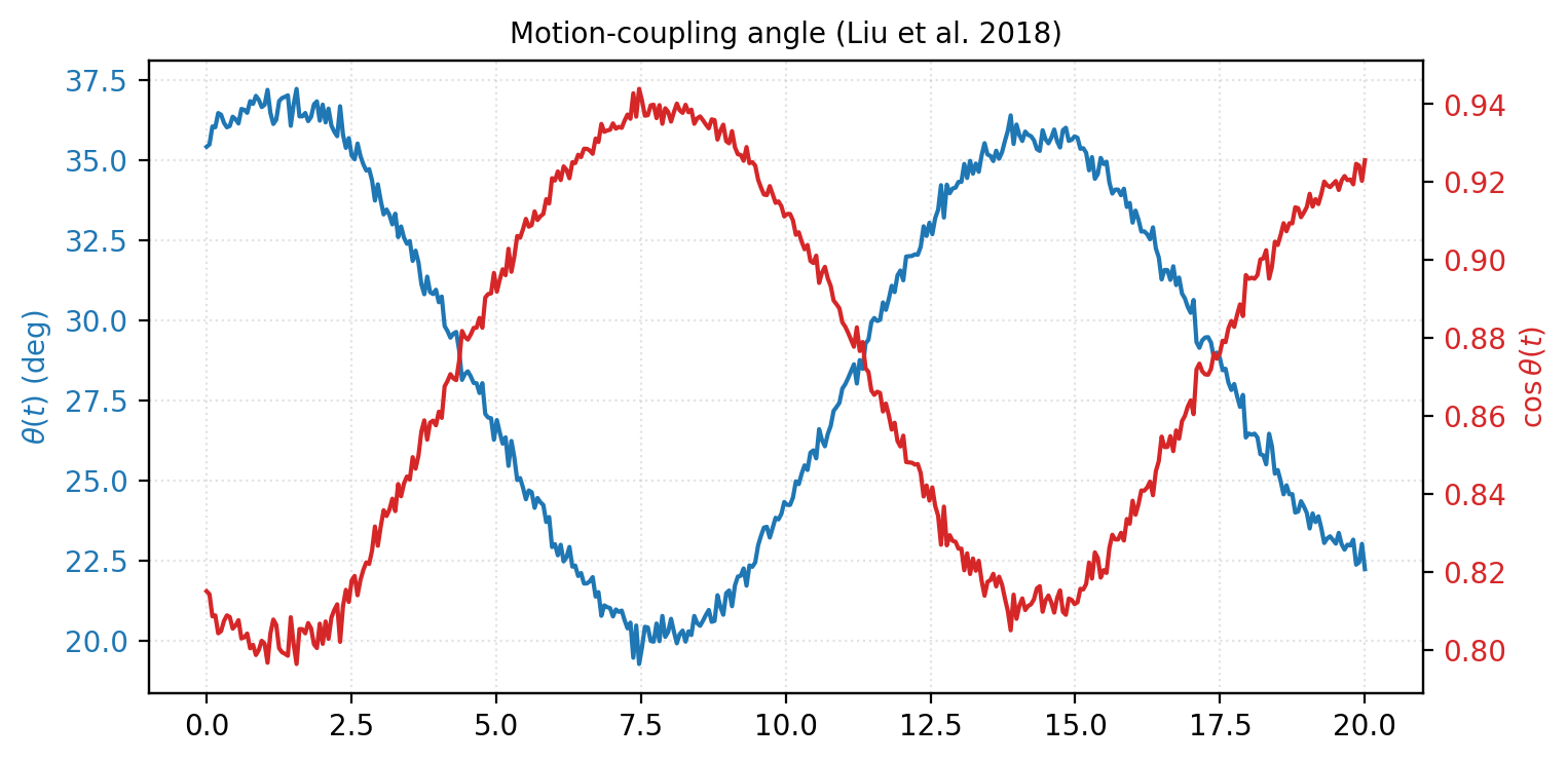
../../_images/user-guide-emtools-afmag-05.png

\(\theta(t)\) (blue, left axis) and \(\cos\theta(t)\) (red, right axis) move in lockstep but in opposite directions, exactly as their definition requires: whenever the coil normal swings further from the field direction, \(\theta\) grows and \(\cos\theta\) shrinks. Because simulate_motion_induced_voltage() differentiates \(\cos\theta(t)\), the slope of the red curve – not its absolute level – is what actually predicts the noise voltage: the noise is largest exactly where the red curve crosses its midline fastest, near \(t\approx4\) and \(t\approx11\) seconds above, and smallest near the peaks and troughs, where the curve momentarily flattens. This is the mechanism behind Liu et al. (2018)’s own reported result: the predicted noise tracks the rate of attitude change, not the raw attitude angle itself.

11.14.7. Motion-Coupling Susceptibility#

Full time-domain correction needs a real attitude and voltage time series, which no bundled dataset carries – see Common Pitfalls below. What the physics above does give, without any time series at all, is a purely geometric answer to “how exposed is this survey’s low-frequency band to motion noise, given a typical amount of platform wobble and this region’s geomagnetic geometry”. motion_susceptibility_table sweeps a nominal attitude-amplitude envelope through motion_coupling_cosine and reports the resulting \(\cos\theta\) swing per station:

>>> from pycsamt.emtools import motion_susceptibility_table
>>> sus = motion_susceptibility_table(
...     sites,
...     inclination=-62.0,
...     declination=-20.0,
...     roll_amplitude_deg=8.0,
...     pitch_amplitude_deg=5.0,
... )
>>> sus["susceptibility_score"].unique()
array([0.12598292])

Every station reports the same score here – a direct consequence of the model, not a plotting artefact: the score depends only on the shared inclination, declination, and attitude amplitude passed in, none of which vary by station in this call. A real survey with per-line attitude logs and a spatially varying geomagnetic field would show real station-to-station variation instead. plot_motion_susceptibility_map places the score at each station’s real coordinates, which is still useful even when the colour itself is uniform, because it shows exactly which part of the survey the score applies to:

>>> from pycsamt.emtools import plot_motion_susceptibility_map
>>> ax = plot_motion_susceptibility_map(
...     sites,
...     inclination=-62.0,
...     declination=-20.0,
...     roll_amplitude_deg=8.0,
...     pitch_amplitude_deg=5.0,
... )
>>> ax.figure.savefig("afmag_susceptibility_map.png", dpi=200, bbox_inches="tight")

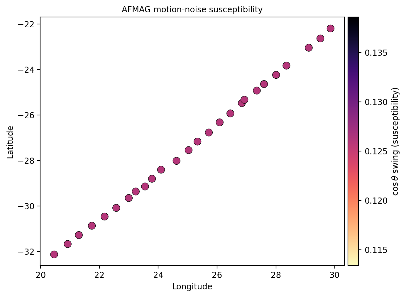
../../_images/user-guide-emtools-afmag-06.png

The map reproduces KAP03’s real southwest-northeast line across southern Africa, confirming the station geometry is genuine even though the colour scale itself carries no per-station information for this particular, geometry-only call.

11.14.8. Flagging A Motion-Susceptible Band#

flag_motion_susceptible_band is the one mutating, Sites-in/Sites-out function in this module. When a station’s susceptibility score exceeds a threshold, it masks (or drops) tipper values in a chosen frequency band – the same ensure_sites/mutation contract as notch_powerline(). This is a QC gate, not a noise-removal algorithm: it flags a plausibly contaminated band for review, rather than attempting the paper’s literal time-domain subtraction against data that was never a time series to begin with.

KAP03’s own real sampling is concentrated below about \(0.1\)Hz, with almost nothing near the historical AFMAG comparator band this function defaults to (\(150\)-\(510\)Hz) – another reminder that this is a ground MT survey being reused for its tipper geometry, not a real AFMAG delivery. The example below instead targets KAP03’s own short-period band, \(0.005\)-\(0.04\)Hz (the same \(25\)-\(200\) second band used for the short-period induction rose on Transfer Functions And Tipper Diagnostics), with a threshold just below the \(0.126\) score computed above so the flag actually triggers:

>>> from pycsamt.emtools import flag_motion_susceptible_band, plot_afmag_correction_comparison
>>> corrected = flag_motion_susceptible_band(
...     sites,
...     inclination=-62.0,
...     declination=-20.0,
...     roll_amplitude_deg=8.0,
...     pitch_amplitude_deg=5.0,
...     threshold=0.1,
...     band_hz=(0.005, 0.04),
... )
>>> before_n = table["tilt_real_deg"].notna().sum()
>>> after_n = afmag_tilt_angles(corrected)["tilt_real_deg"].notna().sum()
>>> print("finite tilt values -- before:", before_n, " after:", after_n)
finite tilt values -- before: 517  after: 336
>>> fig = plot_afmag_correction_comparison(
...     sites,
...     inclination=-62.0,
...     declination=-20.0,
...     roll_amplitude_deg=8.0,
...     pitch_amplitude_deg=5.0,
...     threshold=0.1,
...     band_hz=(0.005, 0.04),
... )
>>> fig.savefig("afmag_correction_comparison.png", dpi=200, bbox_inches="tight")

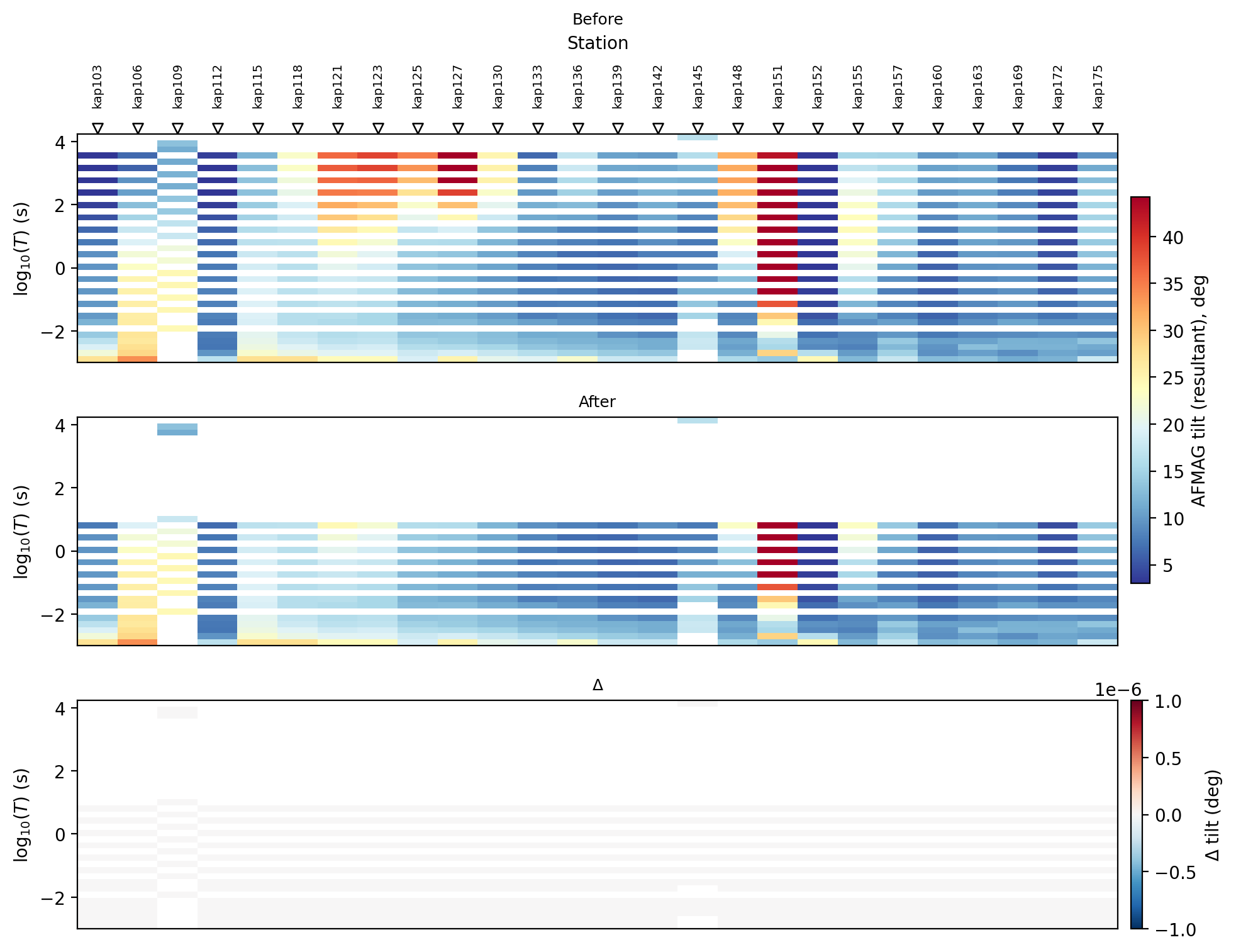
../../_images/user-guide-emtools-afmag-07.png

181 station-frequency values were masked. In the “After” panel, a horizontal gap opens across every station between roughly \(\log_{10}(T)=1.4\) and \(2.3\) – the \(25\)-\(200\) second band just flagged – while everything above and below it, including kap151’s anomaly, is untouched; the “Delta” panel is correspondingly blank everywhere except numerical noise at the \(10^{-6}\) level. That the anomaly survives outside the flagged band, and only the targeted band changes, is exactly the intended behaviour of a QC gate: it should never quietly alter data outside the region it was told to flag.

11.14.9. Two Response Families, On Real Airborne Data#

Everything above reads a tipper – real or, for KAP03, reused – through the tensor-generation’s real/imaginary decomposition. That is only half the picture: pycsamt.airborne.afmag keeps two AFMAG generations genuinely separate rather than collapsing them into one schema, because they are scientifically different responses, not two configurations of the same one. The historical two-coil comparator [Ward1959] reports a single real tilt/deflection angle per frequency – no input or output channels, no polarization-ellipse decomposition possible at all. Modern tensor AFMAG/AirMt systems report a complex Interstation transfer function, relating the fixed ground-reference horizontal field to the airborne three-component field,

(1)#\[\begin{split}\begin{pmatrix} H_x \\ H_y \\ H_z \end{pmatrix}_{r} = \begin{pmatrix} H_{xx} & H_{xy} \\ H_{yx} & H_{yy} \\ H_{zx} & H_{zy} \end{pmatrix} \begin{pmatrix} H_x \\ H_y \end{pmatrix}_{r_0},\end{split}\]

where \(r\) denotes the airborne receiver and \(r_0\) the Remote reference ground magnetic station. The horizontal sub-block (\(H_{xx}, H_{xy}, H_{yx}, H_{yy}\)) relates airborne to ground horizontal fields directly and stays close to the identity matrix over a magnetically quiet background; the vertical row (\(H_{zx}, H_{zy}\)) is the physically interesting part – exactly the same \(H_z\)-to-horizontal relation a ZTEM tipper describes (ZTEM Total-Divergence, Phase-Rotation, And Map-View Diagnostics), just referenced to a fixed ground station instead of the airborne horizontal field itself. AirborneSite exposes these as two separate accessors, afmag_tilt_deg (the comparator’s scalar angle) and interstation_tensor (AirMt’s \((n_f, 3, 2)\) tensor) – never one generic “AFMAG tipper” slot that would blur which generation produced a given file. No real AFMAG measurement ever reaches Site in the first place: it has no electric-field channel, so emtf_to_edi() deliberately refuses to build an EDI from it. pycsamt.airborne.afmag and AirborneSite exist to carry AFMAG data instead, from raw decoded arrays through to a real, readable survey, without ever forcing it through the EDI bridge, using the two synthetic sample surveys committed under data/AFMAG/.

11.14.10. Building A Comparator Response#

build_original_afmag_line() accepts a NavigationTrack and a real, line-batched tilt array and returns one flight line with one EMTF document per sample. The example below builds a small five-station line with a seeded synthetic anomaly at station S03:

>>> from pycsamt.airborne import NavigationTrack
>>> from pycsamt.airborne.afmag import (
...     OriginalAFMAGSystemSpec, build_original_afmag_line,
... )
>>> rng = np.random.default_rng(7)
>>> nav = NavigationTrack(
...     sample_ids=("S01", "S02", "S03", "S04", "S05"),
...     easting=np.array([0.0, 60.0, 120.0, 180.0, 240.0]),
...     northing=np.zeros(5),
... )
>>> freqs = np.array([150.0, 510.0])
>>> tilt = rng.normal(loc=0.0, scale=2.0, size=(5, 2))
>>> tilt[2, :] += 12.0  # a genuine anomaly at station S03
>>> line = build_original_afmag_line(
...     "DEMO01", nav, tilt, frequency=freqs,
...     system_spec=OriginalAFMAGSystemSpec(),
... )
>>> line.n_records
5
>>> record = line.get_record("S03")
>>> tilt_s03 = record.emtf.get_transfer_function("afmag_tilt").data.reshape(-1)
>>> np.round(tilt_s03, 2)
array([11.09, 10.02])

The comparator reports the tilt directly, in degrees, with no arctan/decomposition step – there is nothing to decompose, since the historical instrument only ever measured this one real number. OriginalAFMAGSystemSpec carries the published descriptive characteristics of the instrument (two crossed coils, a nominal 45-degree tilt and separation, a 1-20000 Hz historical operating band) rather than parser constraints:

>>> OriginalAFMAGSystemSpec()
OriginalAFMAGSystemSpec(historical_frequency_band_hz=tuple([1.0, 20000.0]), typical_frequencies_hz=tuple([150.0, 510.0]), coil_count=2, coil_tilt_deg=45.0, coil_separation_deg=45.0, digital_recording=False, attrs=dict(len=0, keys=[]))

11.14.11. Building An AirMt Response#

build_airmt_line() follows the same shape but for the tensor generation, and additionally accepts an AFMAGReferenceStation describing the fixed ground magnetic reference. Building it also derives, by default, the rotation-invariant Amplification parameter from the two column vectors \(T_1\) (the Hx-input response) and \(T_2\) (the Hy-input response) of the tensor:

(2)#\[\mathbf{K} = \mathbf{T}_1 \times \mathbf{T}_2, \qquad AP = \frac{\mathbf{K} \cdot \mathrm{Re}(\mathbf{K})} {\left|\mathrm{Re}(\mathbf{K})\right|}.\]

>>> from pycsamt.airborne.afmag import (
...     AFMAGReferenceStation, AirMtSystemSpec, build_airmt_line,
...     compute_airmt_amplification_parameter,
... )
>>> from pycsamt.metadata import LocationMeta, SiteMeta
>>> rng = np.random.default_rng(3)
>>> nav = NavigationTrack(
...     sample_ids=("R01", "R02", "R03", "R04"),
...     easting=np.array([0.0, 80.0, 160.0, 240.0]),
...     northing=np.zeros(4),
... )
>>> freqs = np.array([25.0, 100.0, 400.0])
>>> tensor = np.zeros((4, 3, 3, 2), dtype=complex)
>>> for i in range(4):
...     for k in range(3):
...         tensor[i, k, 0, 0] = 1.0
...         tensor[i, k, 1, 1] = 1.0
...         tensor[i, k, 2, 0] = 0.1 + 0.03j if i != 2 else 0.35 + 0.12j
...         tensor[i, k, 2, 1] = 0.02 - 0.01j if i != 2 else 0.08 - 0.05j
>>> tensor += 0.01 * (
...     rng.normal(size=tensor.shape) + 1j * rng.normal(size=tensor.shape)
... )
>>> reference = AFMAGReferenceStation(
...     station_id="DEMO_BASE",
...     site=SiteMeta(
...         site_id="DEMO_BASE",
...         location=LocationMeta(
...             latitude=31.30, longitude=97.15, elevation=4170.0,
...         ),
...     ),
... )
>>> line = build_airmt_line(
...     "DEMO02", nav, tensor, frequency=freqs,
...     reference_station=reference, system_spec=AirMtSystemSpec(),
... )
>>> line.n_records
4
>>> record = line.get_record("R03")
>>> tf = record.emtf.get_transfer_function("interstation_transfer_functions")
>>> np.round(tf.data[0], 3)  # the 25 Hz matrix
array([[ 0.972+0.002j,  0.01 +0.026j],
       [-0.01 +0.015j,  0.983+0.015j],
       [ 0.353+0.1j  ,  0.087-0.053j]])

Station R03 was built with a deliberately stronger vertical row (\(H_{zx} = 0.35 + 0.12j\), versus \(0.1 + 0.03j\) at every other station); the horizontal sub-block stays close to the identity matrix everywhere, matching (1)’s description above. compute_airmt_amplification_parameter() implements (2) directly and matches what build_airmt_line() already attached to every record automatically:

>>> ap_manual = compute_airmt_amplification_parameter(tf.data)
>>> np.round(ap_manual, 4)
array([1.0199+0.0451j, 1.0633+0.0464j, 1.0563+0.04j  ])
>>> ap_stored = record.emtf.get_transfer_function(
...     "airmt_amplification_parameter",
... ).data.reshape(-1)
>>> np.allclose(ap_manual, ap_stored)
True

11.14.12. Reading The Sample Surveys#

data/AFMAG/ carries two synthetic sample surveys, one per generation, forward-modeled from a simplified skin-depth-weighted target on a 1-D background – not a reproduction of either cited paper’s actual field data (every generated file’s Description says so explicitly; see the warning further below). ensure_asites() reads either straight from its directory, mirroring how this page’s earlier sections read a directory of ground EDI files:

>>> from pycsamt.airborne.site import ensure_asites
>>> abitibi = ensure_asites("data/AFMAG/abitibi_on")
>>> yulong = ensure_asites("data/AFMAG/yulong_belt_cn")
>>> len(abitibi), abitibi.technologies
(13, ('afmag_original',))
>>> len(yulong), yulong.technologies
(11, ('afmag_airmt',))
>>> abitibi[0]
AirborneSite(name='AB_001', technology='afmag_original', nfreq=2, coords=(48.25000,-79.30000,305.0))
>>> abitibi[0].freq
array([150., 510.])
>>> np.round(abitibi[0].afmag_tilt_deg, 3)
array([-0.141,  0.367])
>>> yulong.get("YU_006")
AirborneSite(name='YU_006', technology='afmag_airmt', nfreq=6, coords=(31.30359,97.20000,4200.0))
>>> yulong.get("YU_006").interstation_tensor.shape
(6, 3, 2)

abitibi_on mimics a historical Canadian-Shield-style massive-sulphide VMS target, read at Ward’s own two typical comparator frequencies (150, 510 Hz). yulong_belt_cn mimics a porphyry-Cu alteration halo, motivated by [Liu2018]’s treatment of a modern digital AirMt-class system, read at six log-spaced frequencies across the published 20-800 Hz AirMt practical band. Both surveys are single flight lines of otherwise-independent stations – technologies confirms neither file mixes generations, a real, checkable guarantee rather than an assumption.

11.14.13. Tilt Tables From Real Data#

original_afmag_tilt_table() and airmt_tilt_angles() turn either AirborneSites into a tidy pandas.DataFrame, the same sites-in/DataFrame-out shape this page already uses for ground tipper data:

>>> from pycsamt.emtools.afmag import (
...     airmt_tilt_angles, original_afmag_tilt_table,
... )
>>> table1 = original_afmag_tilt_table(abitibi)
>>> table1.shape
(26, 4)
>>> table1[np.isclose(table1["freq"], 150.0)].reset_index(drop=True)
   station   freq    period  tilt_deg
0   AB_001  150.0  0.006667 -0.140700
1   AB_002  150.0  0.006667  0.264722
2   AB_003  150.0  0.006667 -0.476803
3   AB_004  150.0  0.006667  0.346270
4   AB_005  150.0  0.006667  0.668092
5   AB_006  150.0  0.006667  2.406585
6   AB_007  150.0  0.006667  0.474760
7   AB_008  150.0  0.006667 -2.821927
8   AB_009  150.0  0.006667 -0.093457
9   AB_010  150.0  0.006667  0.078964
10  AB_011  150.0  0.006667 -0.521222
11  AB_012  150.0  0.006667  0.209250
12  AB_013  150.0  0.006667  1.071325
>>> table2 = airmt_tilt_angles(yulong)
>>> table2.shape
(66, 8)
>>> list(table2.columns)
['station', 'freq', 'period', 'tilt_real_deg', 'tilt_real_azimuth_deg', 'tilt_imag_deg', 'tilt_imag_azimuth_deg', 'tilt_resultant_deg']

table1’s tilt_deg column is signed, straight from the comparator: it crosses zero between AB_006 (\(+2.4^\circ\)) and AB_008 (\(-2.8^\circ\)), the classic AFMAG signature of a conductor centred between two stations. table2’s columns come from the same real/imaginary decomposition used earlier for a ground tipper (\(\arctan|T_c|\)), applied instead to the tensor’s \((H_{zx}, H_{zy})\) row – so, unlike tilt_deg, tilt_real_deg and tilt_resultant_deg are magnitudes (an arctan of a hypotenuse, never negative); the target’s position shows up in the paired _azimuth_deg column instead, taken up next.

11.14.14. Dual-Frequency Crossover Profile#

The comparator’s actual field product is not a single-frequency curve – Ward’s own instrument always recorded 150 and 510 Hz together, and his worked interpretation (1959, Fig. 16 and Results section) reads three things off that pair jointly: the along-line crossover where the signed tilt changes sign at each frequency (the conductor axis), the shift between the two crossovers (inhomogeneity along the body), and the peak-to-peak amplitude ratio between the two frequencies, a semi-quantitative conductivity estimate ranging from 0 (very poor) toward 1 (excellent). His own worked example on a pyrite-pyrrhotite body gives \((7+35)/(23+34)=0.74\). original_afmag_conductor_diagnostics() reproduces exactly this – and only this: Ward’s further depth, depth-extent, and dip estimates all need a scale-model calibration curve the paper does not give in closed form, so, matching this module’s standing policy of never inventing a formula the cited literature does not itself supply, they are not computed here.

>>> from pycsamt.emtools.afmag import original_afmag_conductor_diagnostics
>>> diag = original_afmag_conductor_diagnostics(abitibi)
>>> round(diag["crossover_low_m"], 1), round(diag["crossover_high_m"], 1)
(369.3, 353.3)
>>> round(diag["crossover_shift_m"], 1)
-16.0
>>> round(diag["peak_to_peak_low"], 2), round(diag["peak_to_peak_high"], 2)
(5.23, 7.12)
>>> round(diag["peak_to_peak_ratio"], 2)
0.73

abitibi_on’s synthetic ratio, \(0.73\), lands almost exactly on Ward’s own worked value of \(0.74\) – not by construction (the two surveys share no parameters), simply because both describe a single compact conductor with a real, physically-consistent frequency response. The two crossovers sit only 16 m apart out of a 720 m line, i.e. the target reads as laterally coherent, not inhomogeneous, between the two frequencies. plot_original_afmag_dual_frequency_profile() draws exactly the figure this table describes:

>>> from pycsamt.emtools.afmag import plot_original_afmag_dual_frequency_profile
>>> ax = plot_original_afmag_dual_frequency_profile(abitibi)
>>> ax.figure.savefig("user-guide-emtools-afmag-08.png", dpi=200, bbox_inches="tight")

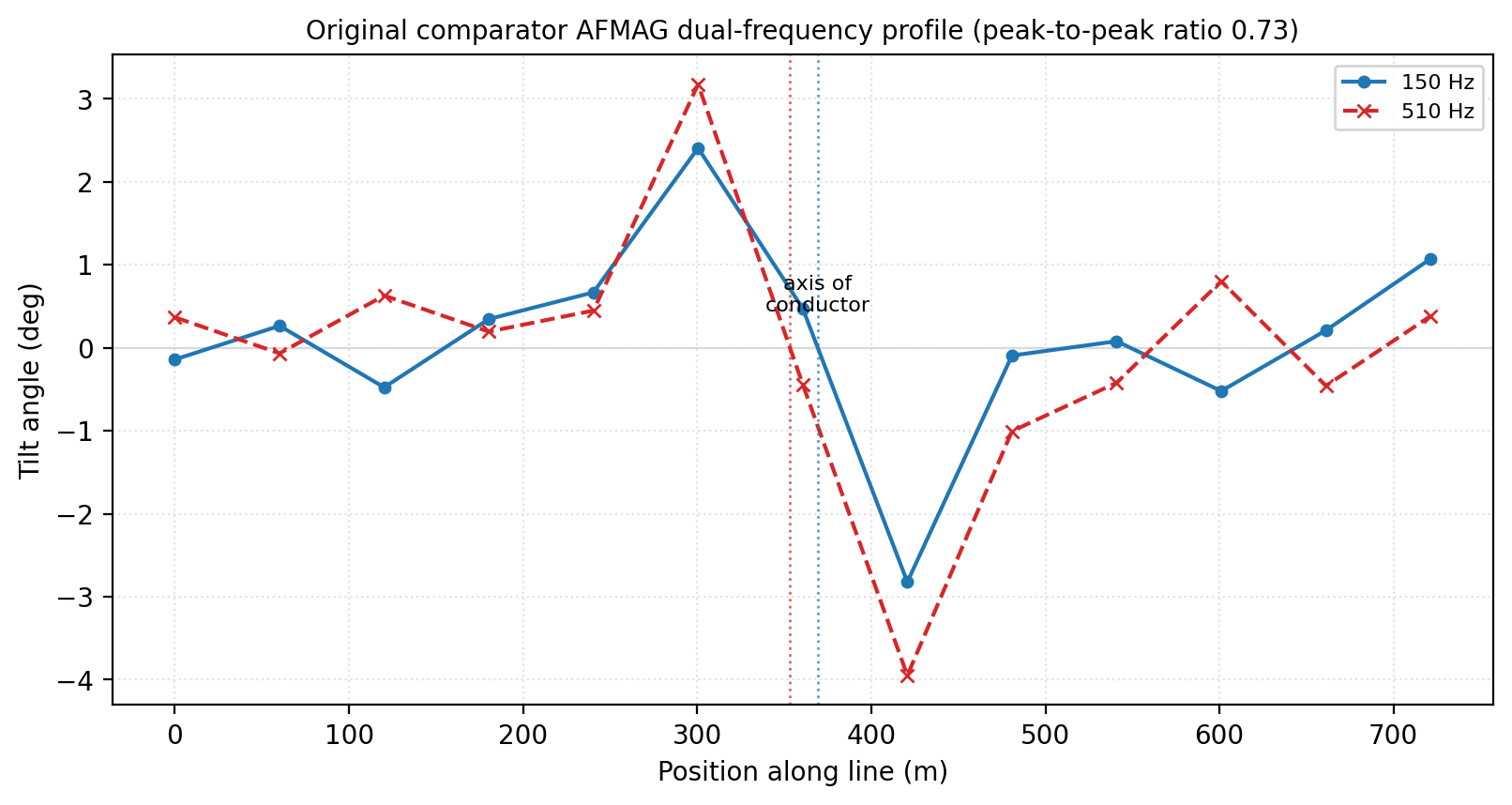
Dual-frequency comparator tilt profile, abitibi_on – the same 150/510 Hz overlay convention as Ward (1959) Fig. 16, dotted vertical lines marking each frequency’s crossover.#

The two curves trace the same shape – a broad rise to \(+2.4^\circ\)/\(+3.2^\circ\) at AB_006, a sharp fall to \(-2.8^\circ\)/\(-4.0^\circ\) at AB_008 – with 510 Hz consistently the larger swing, matching \(0.73<1\): the higher frequency couples more strongly to this shallow, 100 m-deep synthetic target, exactly the frequency-dependence a real skin-depth-limited response should show.

11.14.15. AirMt Tilt Pseudosection#

The dual-frequency overlay above works because the comparator only ever has two frequencies to compare. AirMt has no such fixed pair – yulong_belt_cn carries six log-spaced frequencies across the published 20-800 Hz practical band – so the natural presentation is not one more overlay but the same station-x-log-period pseudosection every other airborne technology in this project already gets (plot_ztem_divergence_psection(), plot_mobilemt_conductivity_psection(), plot_afmag_tilt_psection() for the ground-tipper-shaped case above). Before this section, airmt_tilt_angles() had no pseudosection of its own at all – only the single-frequency plot_airmt_tilt_profile() – so plot_airmt_tilt_psection() closes that real gap:

>>> from pycsamt.emtools.afmag import plot_airmt_tilt_psection
>>> ax = plot_airmt_tilt_psection(yulong)
>>> ax.figure.savefig("user-guide-emtools-afmag-09.png", dpi=200, bbox_inches="tight")

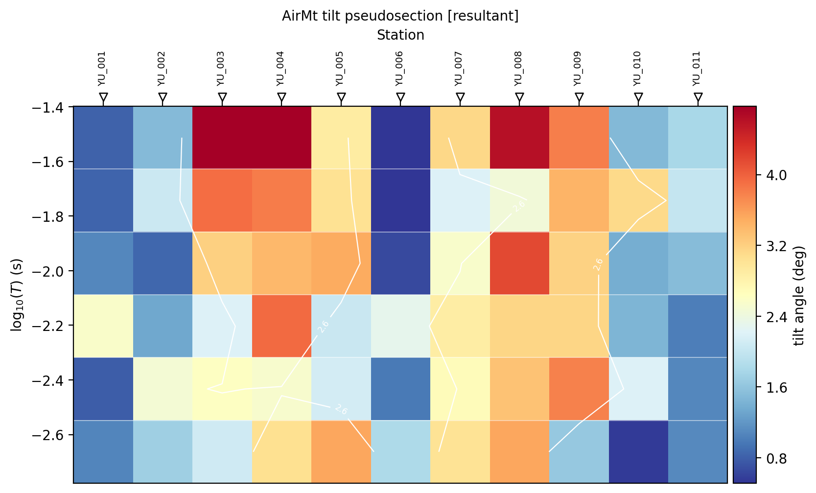
../../_images/user-guide-emtools-afmag-09.png — AirMt tilt-magnitude pseudosection, `yulong_belt_cn`, all six frequencies at once.#

Two overlays on top of the raw grid, on by default (show_grid/show_contour), match the imshow/contour convention pycsamt.emtools.fieldzone’s own pseudosection already uses: thin white lines mark every station/period cell boundary, and one white contour line traces the field’s own median value across the grid, with its numeric level labelled inline. Only a single contour level is drawn here (n_contour_levels=3 by default, i.e. one interior level) rather than several – with five, the contour tangles into a cluttered web on a grid this coarse and noisy, which would misrepresent a genuinely blocky measurement as smoothly resolved structure; one median line stays legible and honestly reads as a boundary, not a resolved gradient.

Unlike the comparator’s clean two-frequency crossover, the pseudosection is visibly noisier station to station and period to period – a real consequence of this module’s construction, not an artifact of the plot: airmt_tilt_angles reads tilt_real_deg, an \(\arctan\) magnitude (see the previous section), so it folds the target signal and the tensor’s own instrument-noise floor together into one always-positive number with no sign to average against. The contour line still helps here: it separates a warmer cluster around YU_003/YU_004/YU_008/YU_009 from a cooler one at both line ends, tracing the same broad pattern the raw colours already show but as one continuous boundary rather than a station-by-station read.

11.14.16. Azimuth Across The Target#

The pseudosection above cannot show a sign the way the comparator’s crossover does – tilt_real_deg is a magnitude by construction. The direction that magnitude points is a separate column, tilt_real_azimuth_deg, with no dedicated plotting function, so the figure below is built directly from table2:

>>> f0 = sorted(table2["freq"].unique())[2]  # the 89 Hz frequency
>>> sub = table2[table2["freq"] == f0].reset_index(drop=True)
>>> sub[["station", "tilt_real_deg", "tilt_real_azimuth_deg"]]
   station  tilt_real_deg  tilt_real_azimuth_deg
0   YU_001       2.002124             178.649894
1   YU_002       1.300724             155.754386
2   YU_003       1.767688            -140.288451
3   YU_004       3.659670            -172.402245
4   YU_005       1.407168            -139.967361
5   YU_006       1.927480              18.022650
6   YU_007       2.453867              -5.791069
7   YU_008       2.951837              -1.927638
8   YU_009       2.305912              16.836155
9   YU_010       1.018292              12.574053
10  YU_011       0.724839             168.278878
>>> stations = sub["station"].tolist()
>>> azimuth = sub["tilt_real_azimuth_deg"].to_numpy()
>>> fig, ax = plt.subplots(figsize=(9.5, 3.8))
>>> x = np.arange(len(stations))
>>> _ = ax.axhline(0.0, color="0.85", lw=0.8)
>>> _ = ax.plot(x, azimuth, marker="o", lw=1.6, color="tab:orange")
>>> _ = ax.set_xticks(x)
>>> _ = ax.set_xticklabels(stations, rotation=45, ha="right", fontsize=8)
>>> _ = ax.set_ylabel("tilt_real_azimuth_deg")
>>> _ = ax.set_title(f"AirMt real-tilt azimuth along the line at {f0:.1f} Hz")
>>> fig.savefig("user-guide-emtools-afmag-10.png", dpi=200, bbox_inches="tight")

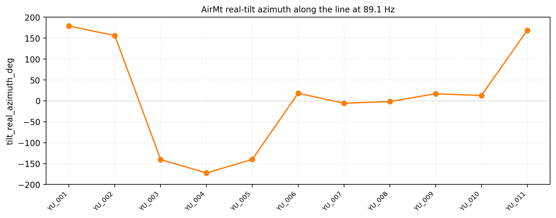
../../_images/user-guide-emtools-afmag-10.png — AirMt real-tilt azimuth along the `yulong_belt_cn` line, same 89 Hz frequency as the pseudosection above.#

This is the tensor generation’s version of the comparator’s sign flip: azimuth sits near \(\pm 180^\circ\) from YU_001 to YU_005, flips to near \(0^\circ\) from YU_006 onward, and flips back at the line’s far end (YU_011). Read together with the magnitude profile above, the target sits between YU_004/YU_005 and YU_006 – the same crossover signature the comparator shows directly through a sign change, recovered here from a magnitude and an azimuth column instead.

11.14.17. Flight-Line Geometry#

AirMt’s tensor is referenced to a fixed ground station, so its geometry – how far the reference sits from the flight line – is itself worth inspecting, again with no dedicated plot function:

>>> lats = [s.coords[0] for s in yulong]
>>> lons = [s.coords[1] for s in yulong]
>>> names = [s.sample_id for s in yulong]
>>> ref_lat, ref_lon = 31.304492, 97.190538  # from EMTF.metadata["notes"]
>>> fig, ax = plt.subplots(figsize=(6.0, 6.0))
>>> _ = ax.plot(lons, lats, "-", color="0.7", lw=1.2)
>>> _ = ax.scatter(lons, lats, c="tab:blue", s=45, label="flight line")
>>> _ = ax.scatter([ref_lon], [ref_lat], marker="*", s=220, color="tab:red",
...                 label="ground magnetic reference")
>>> _ = ax.set_xlabel("Longitude")
>>> _ = ax.set_ylabel("Latitude")
>>> _ = ax.legend(loc="lower left", fontsize=8)
>>> fig.savefig("user-guide-emtools-afmag-11.png", dpi=200, bbox_inches="tight")

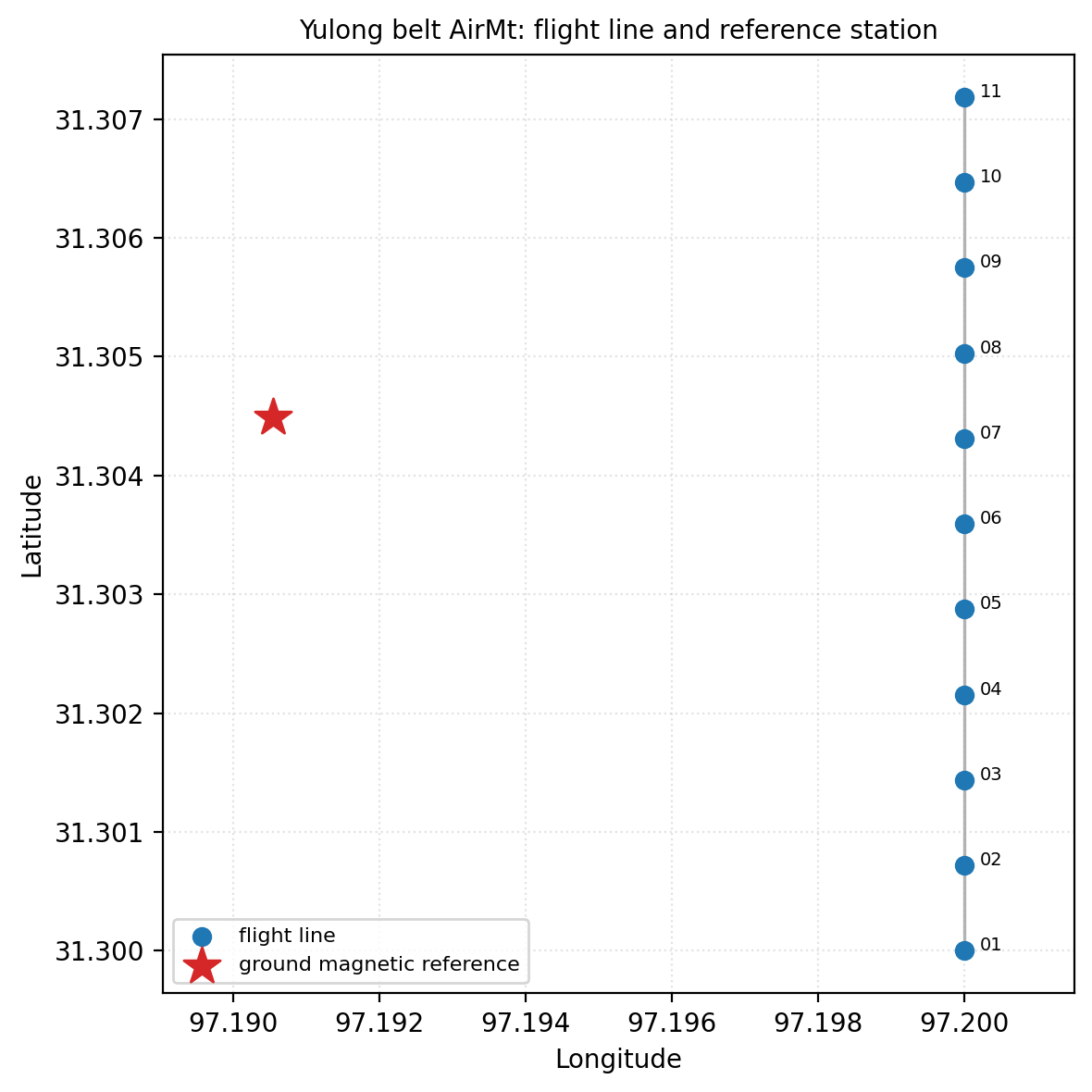
../../_images/user-guide-emtools-afmag-11.png — `yulong_belt_cn`’s north-south flight line and its fixed ground magnetic reference station, roughly 900 m west of the line.#

The reference station’s latitude/longitude are not exposed directly on AirborneSite – only its identifier is (site.processing.remote_reference.site), matching AFMAGReferenceStation’s own role as a processing-time input rather than a flight-line sample. Its coordinates were instead read from EMTF.metadata["notes"]["AFMAG"], one of the presentation-metadata blocks build_airmt_line() writes and that does round-trip through EMTF-XML (unlike EMTF.attrs, which does not).

11.14.18. Amplification Parameter Behavior#

It is tempting to expect Amplification parameter to spike over the target the way the tensor’s raw \(H_{zx}\) does. The real data say otherwise:

>>> picks = ["YU_002", "YU_006", "YU_009"]
>>> fig, (ax1, ax2) = plt.subplots(1, 2, figsize=(11.0, 4.0))
>>> for name in picks:
...     site = yulong.get(name)
...     freq, ap = site.freq, site.afmag_amplification_parameter
...     ax1.plot(freq, np.abs(ap), marker="o", label=name)
...     ax2.plot(freq, np.degrees(np.angle(ap)), marker="o", label=name)
>>> _ = ax1.axhline(1.0, color="0.75", ls="--")
>>> ax1.set_xscale("log")
>>> _ = ax1.set_ylabel(r"$|AP|$")
>>> _ = ax1.legend(fontsize=8)
>>> _ = ax2.axhline(0.0, color="0.75", ls="--")
>>> ax2.set_xscale("log")
>>> _ = ax2.set_ylabel(r"$\arg(AP)$ (deg)")
>>> _ = ax2.legend(fontsize=8)
>>> fig.savefig("user-guide-emtools-afmag-12.png", dpi=200, bbox_inches="tight")

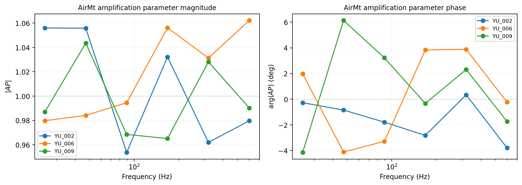
../../_images/user-guide-emtools-afmag-12.png — AirMt amplification-parameter magnitude and phase at three stations spanning the target (`YU_002`, off-target; `YU_006`, near-target; `YU_009`, off-target on the other side).#

|AP| stays within about \(\pm 6\%\) of unity at every station and frequency, with no systematic separation between the near-target and off-target stations picked above – consistent with (2)’s construction: \(AP\) is a normalized projection of \(T_1 \times T_2\) onto its own real part, not a raw amplitude, so it is close to rotation- and scale-invariant by design. That makes it a poor choice for flagging where a target is (the vertical row itself, or the magnitude/azimuth pair used above, already do that job); its intended role is instead as a discriminator of tensor character – e.g. distinguishing a genuine, coherent interstation response from a degenerate or noisy one where \(|\mathrm{Re}(\mathbf{K})|\) collapses toward zero (see zero_policy on compute_airmt_amplification_parameter()). Expecting it to behave like an anomaly map is a real, easy misreading of a rotation-invariant quantity – worth stating plainly rather than leaving a reader to assume it from the name alone.

Warning

Every file under data/AFMAG/ is synthetic, forward-modeled from a simplified skin-depth-weighted analytic approximation – not a vendor delivery sample and not a reproduction of either cited paper’s actual field data. Each generated EMTF.description states this explicitly, and it is repeated here so the numbers on this page are never mistaken for real field measurements. No proprietary AFMAG/AirMt archive format is parsed anywhere in pyCSAMT; pycsamt.airborne.afmag only maps already-decoded arrays onto the common model.

11.14.19. Common Pitfalls#

Do not treat KAP03’s tilt-angle figures on this page as a real AFMAG survey result. They demonstrate the tilt-angle transformation correctly, on real tipper data, but the underlying survey is ground MT, not airborne AFMAG.

Do not fabricate precision for geomagnetic inclination/declination. The values used above are representative round numbers for the region, clearly not an IGRF lookup; a real survey should use its own site- and epoch-correct values.

Do not expect flag_motion_susceptible_band’s default \(150\)-\(510\)Hz band to do anything useful on a dataset whose real frequency coverage does not reach it – check with afmag_tilt_angles()’s own freq column before assuming a call silently failed.

Do not expect this module to perform the paper’s literal time-domain noise subtraction. euler_rotation_matrix through simulate_motion_induced_voltage are the reusable physics for whoever has a real attitude and voltage time series; a frequency-domain Sites/AirborneSites object has no time axis to run that subtraction on, so flag_motion_susceptible_band offers the QC-gate alternative instead.

Do not expect a tilt-angle-derived apparent resistivity or conductivity from this module. Unlike full MT, nothing in Ward (1959) or Liu et al. (2018) provides a simple closed form for that conversion, so none is invented here.

Do not treat every file under data/AFMAG/ as a real survey either – both abitibi_on and yulong_belt_cn are synthetic, exactly like KAP03’s motion-coupling demonstration is synthetic, just for a different reason (no AFMAG vendor has supplied pyCSAMT with a real delivery at all; see the warning in Two Response Families, On Real Airborne Data above).

Do not expect Amplification parameter to behave like an anomaly map. It is a normalized, close-to-rotation-invariant projection by construction ((2)), not a raw amplitude – see “Amplification Parameter Behavior” above for the real data showing this directly.

11.14.20. Recommended Workflow#

A complete AFMAG diagnostic pass on KAP03’s ground tipper reads the tilt profile, checks its period behaviour, reads one station’s polar view, characterizes the motion-coupling physics (both the sensitivity grid and one illustrative segment), maps susceptibility, and finally checks a flagged-band comparison – each already shown individually above. The dropdown below is that same sequence as one self-contained script, reproducing every KAP03 figure on this page end to end:

Read that part of the page in this order: the profile and pseudosection identify which station and period range are anomalous (kap151, essentially every period); the polar view checks whether that anomaly is a coherent physical response or scatter (coherent, here); the sensitivity grid and illustrative segment characterize the motion-coupling physics itself, independent of any survey; the susceptibility map ties that physics to KAP03’s own geometry; and the correction comparison confirms that flagging a motion-susceptible band changes only the targeted band, leaving the real anomaly at kap151 untouched.

The second dropdown reproduces every real-airborne-data figure from Two Response Families, On Real Airborne Data onward, on abitibi_on and yulong_belt_cn:

11.14.21. References#

The AFMAG tilt-angle concept and its historical instrument characteristics follow [Ward1959]. The motion-coupling rotation-matrix method, its Euler-angle convention, the reported small-angle test amplitude used in the synthetic example above, and the tensor AirMt generation and survey setting synthesized for yulong_belt_cn all follow [Liu2018]. The KAP03 survey used throughout the first part of this page for its real tipper geometry is the same profile documented in Transfer Functions And Tipper Diagnostics.