
11.16. MobileMT Admittance, Apparent Conductivity, And Skew Diagnostics#
Every method covered so far in this section – AFMAG Tilt-Angle Diagnostics And Motion-Coupling Physics and ZTEM Total-Divergence, Phase-Rotation, And Map-View Diagnostics – is, once the ground reference is fixed, a magnetic-field-to-magnetic-field transfer function: a tipper or an interstation tensor, never an impedance. MobileMT (Prikhodko et al. 2022) breaks that pattern deliberately: its ground reference is a fixed electric dipole pair (\(E_x, E_y\)) rather than a second magnetic station, giving a complex admittance tensor that is the reciprocal of the classical MT impedance, \(Y = Z^{-1}\), in the limit where the airborne and ground sensors are co-located. Airborne Natural-Source EM: AFMAG, ZTEM, And MobileMT derives this relationship in full, including the theoretical apparent-conductivity formula this page uses; this page focuses on the practical side – loading real MobileMT data, reading its admittance and derived diagnostics, and interpreting them on two synthetic surveys.
pycsamt.emtools.mobilemt carries MobileMT data through
AirborneEMDataset rather than through
Site, for the same reason ZTEM/AFMAG avoid
the EDI bridge: an EDI file has nowhere honest to put a ground
electric reference alongside an airborne magnetic response.
ensure_mobilemt_dataset() accepts an
AirborneEMDataset/
AirborneEMLine directly, or anything
ensure_asites() does – an
AirborneSites/
AirborneSite, or a bare path/directory
of EMTF-XML files – regrouping the latter into flight lines
automatically.
Two synthetic sample surveys, committed under data/mobileMT/,
demonstrate this page: flammefjeld_greenland, loosely inspired by
Zhdanov et al. (2024)’s MobileMT/TMI survey over a Climax-style
porphyry molybdenum-copper breccia pipe in East Greenland, and
timiskaming_kimberlite_on, loosely inspired by Prikhodko et al.
(2022)’s survey over the KL-22 kimberlite pipe at Lake Timiskaming,
Ontario. Both are single 12-station flight lines sampled at the same
ten log-spaced frequencies from 25 Hz to 12,000 Hz:
>>> from pycsamt.emtools.mobilemt import ensure_mobilemt_dataset
>>> flammefjeld = ensure_mobilemt_dataset("data/mobileMT/flammefjeld_greenland")
>>> flammefjeld.n_records
12
>>> line = next(flammefjeld.iter_lines())
>>> line.navigation.sample_ids
('FL_001', 'FL_002', 'FL_003', 'FL_004', 'FL_005', 'FL_006', 'FL_007', 'FL_008', 'FL_009', 'FL_010', 'FL_011', 'FL_012')
11.16.1. Admittance Along The Flight Line#
admittance_table() reads every
sample’s admittance tensor into one tidy table – real/imaginary parts
of the horizontal 2x2 block (\(Y_{xx}, Y_{xy}, Y_{yx}, Y_{yy}\))
and the vertical-field row (\(Y_{hzx}, Y_{hzy}\)), plus the
vendor-delivered native apparent conductivity when present:
>>> from pycsamt.emtools.mobilemt import admittance_table
>>> df = admittance_table(flammefjeld)
>>> df.shape
(120, 18)
>>> df.columns.tolist()
['line_id', 'sample_id', 'x_m', 'freq_hz', 'period_s', 'Yxx_real', 'Yxx_imag', 'Yxy_real', 'Yxy_imag', 'Yyx_real', 'Yyx_imag', 'Yyy_real', 'Yyy_imag', 'Yhzx_real', 'Yhzx_imag', 'Yhzy_real', 'Yhzy_imag', 'apparent_conductivity_native_Sm']
12 stations x 10 frequencies gives 120 rows, one admittance tensor
each. plot_mobilemt_admittance_profile()
plots any one entry – or, with component="det", the horizontal
2x2 determinant that the apparent-conductivity formula below is built
from – along the flight line at a chosen frequency:
>>> from pycsamt.emtools.mobilemt import plot_mobilemt_admittance_profile
>>> ax = plot_mobilemt_admittance_profile(flammefjeld, component="det", part="abs", frequency_hz=390.0)
>>> ax.figure.savefig("user-guide-emtools-mobilemt-01.png", dpi=200, bbox_inches="tight")
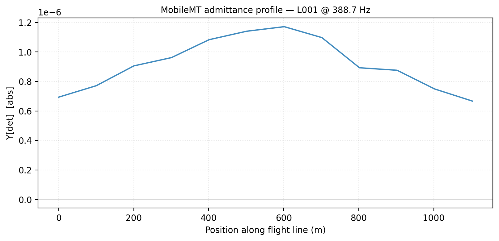
\(|\det Y|\) along the flight line at 388.7 Hz,
flammefjeld_greenland.#
The determinant amplitude rises smoothly from the profile’s ends toward a broad maximum near 500-600 m and falls away again – the along-line signature of the synthetic conductive breccia-pipe target centred on the profile, not an instrument artefact or a sharp edge effect. Because \(|\det Y|\) scales with the inverse of resistivity (see (3)), a higher determinant here means lower resistivity, i.e. a more conductive subsurface directly beneath the peak.
11.16.2. Theoretical Apparent Conductivity Versus The Vendor-Delivered Product#
admittance_determinant_table() turns
that determinant into a physical apparent conductivity and phase using
(3), and reports the vendor-delivered
native product alongside it for direct comparison:
>>> from pycsamt.emtools.mobilemt import admittance_determinant_table
>>> dfd = admittance_determinant_table(flammefjeld)
>>> target = sorted(dfd["freq_hz"].unique())[4]
>>> round(float(target), 1)
388.7
>>> sub = dfd[dfd["freq_hz"] == target].sort_values("x_m")
>>> sub["theoretical_rho_a_ohm_m"].round(0).tolist()
[742.0, 667.0, 568.0, 535.0, 475.0, 451.0, 439.0, 469.0, 576.0, 587.0, 687.0, 771.0]
At 388.7 Hz, the theoretical resistivity and the two conductivity columns read:
Sample |
\(x\) (m) |
\(\rho_a\) theoretical (\(\Omega\cdot\)m) |
\(\sigma_a\) theoretical (S/m) |
\(\sigma_a\) native (S/m) |
|---|---|---|---|---|
FL_001 |
0 |
741.7 |
0.0013 |
0.0013 |
FL_002 |
100 |
667.1 |
0.0015 |
0.0014 |
FL_003 |
200 |
568.1 |
0.0018 |
0.0016 |
FL_004 |
301 |
534.9 |
0.0019 |
0.0019 |
FL_005 |
401 |
475.0 |
0.0021 |
0.0021 |
FL_006 |
501 |
451.1 |
0.0022 |
0.0023 |
FL_007 |
601 |
439.2 |
0.0023 |
0.0023 |
FL_008 |
702 |
468.8 |
0.0021 |
0.0021 |
FL_009 |
802 |
576.2 |
0.0017 |
0.0019 |
FL_010 |
902 |
587.3 |
0.0017 |
0.0016 |
FL_011 |
1002 |
686.8 |
0.0015 |
0.0015 |
FL_012 |
1103 |
771.1 |
0.0013 |
0.0013 |
The theoretical resistivity bottoms out at 439 \(\Omega\cdot\)m
under station FL_007 (601 m along the line) against a host of roughly
740-770 \(\Omega\cdot\)m at the profile’s ends – consistent
with Zhdanov et al. (2024)’s description of a conductive alteration
halo over a resistive core, and close to the 800
\(\Omega\cdot\)m host value the synthetic model was built from.
More importantly, theoretical_sigma_a_Sm (pyCSAMT’s own
co-located-sensor-limit formula) and
apparent_conductivity_native_Sm (the vendor-delivered field, read
back from the survey file) agree to within a few percent at every
station – exactly what (3)’s derivation
predicts, and a useful sanity check to run on any new delivery before
trusting either column.
Note
apparent_conductivity_native_Sm is recovered from
EMTF.metadata["notes"]["MobileMT"]["ApparentConductivitySm"] –
the one part of an EMTF-XML document that survives a write/read
round trip losslessly as free text, since
fields (an in-memory-only
attribute) has no EMTF-XML representation of its own. A real vendor
delivery that stores its processed conductivity elsewhere in the
file, or not at all, will report nan in this column rather than
raise an error – always check for that before comparing it against
the theoretical column.
plot_mobilemt_conductivity_psection()
images either source as a station-versus-log-period pseudosection.
Plotting both with the same colour limits makes the agreement visible
directly rather than only in the table above:
>>> from pycsamt.emtools.mobilemt import plot_mobilemt_conductivity_psection
>>> import matplotlib.pyplot as plt
>>> fig, (ax1, ax2) = plt.subplots(1, 2, figsize=(15.0, 5.2), sharey=True)
>>> _ = plot_mobilemt_conductivity_psection(flammefjeld, source="theoretical", clim=(0.0012, 0.0023), ax=ax1)
>>> _ = plot_mobilemt_conductivity_psection(flammefjeld, source="native", clim=(0.0012, 0.0023), ax=ax2)
>>> fig.savefig("user-guide-emtools-mobilemt-02.png", dpi=200, bbox_inches="tight")
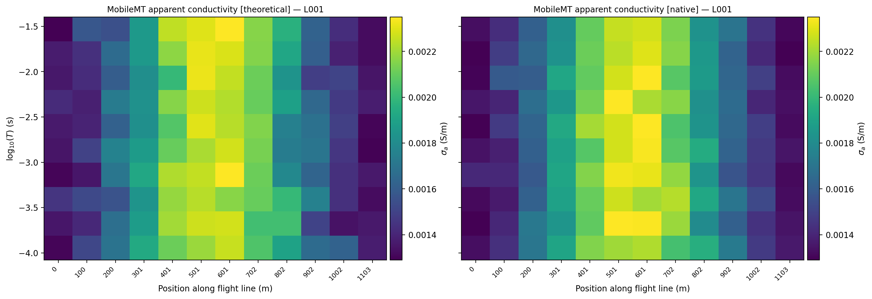
Apparent conductivity, flammefjeld_greenland: pyCSAMT’s
theoretical determinant formula (left) against the vendor-delivered
native field (right), same colour scale.#
The two panels are visually indistinguishable: the same bright, conductive band sits over stations FL_005-FL_008 in both, at every period. That agreement is the practical payoff of (3)’s co-located-sensor derivation – when it holds, either column is a reliable apparent-conductivity product, and disagreement between them on a real survey is itself a diagnostic (of a genuinely non-co-located reference geometry, or of a processing difference) worth investigating rather than ignoring.
11.16.3. Skew: Departure From An Ideal Admittance Tensor#
admittance_skew_table() applies a
Swift (1967)-style skew ratio to the horizontal 2x2 admittance
sub-block, (4) – the same diagnostic
already used for the impedance tensor elsewhere in pyCSAMT (see
Dimensionality, Distortion, And The Phase Tensor), by direct algebraic analogy.
Unlike the apparent-conductivity formula above, skew needs no physical
constant and is safe to compute from any admittance tensor, co-located
or not:
>>> from pycsamt.emtools.mobilemt import admittance_skew_table, plot_mobilemt_skew_profile
>>> timiskaming = ensure_mobilemt_dataset("data/mobileMT/timiskaming_kimberlite_on")
>>> dfs = admittance_skew_table(timiskaming)
>>> round(float(dfs["skew"].mean()), 3), round(float(dfs["skew"].max()), 3)
(0.048, 0.105)
>>> ax = plot_mobilemt_skew_profile(timiskaming, frequency_hz=770.0)
>>> ax.figure.savefig("user-guide-emtools-mobilemt-03.png", dpi=200, bbox_inches="tight")
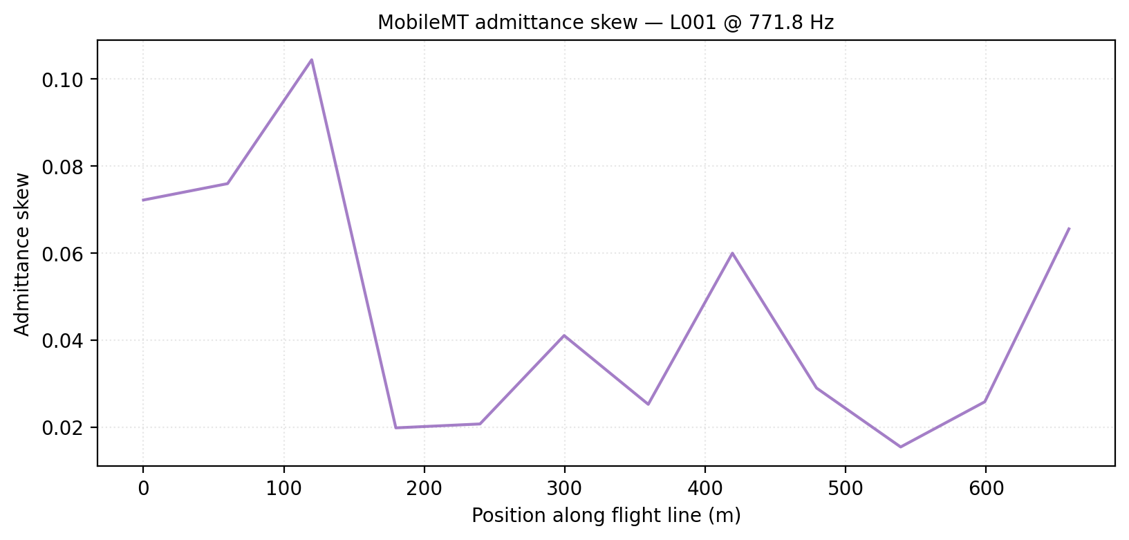
Admittance skew at 771.8 Hz, timiskaming_kimberlite_on.#
Unlike the apparent-conductivity pseudosections above, this profile
has no clean relationship to the kimberlite target centred near
300-360 m: it wanders between roughly 0.02 and 0.10 with no systematic
dip or rise over the conductive zone. That is expected, not a defect
– timiskaming_kimberlite_on’s diagonal admittance terms are built
from independent per-station, per-frequency synthetic noise rather
than from any structural distortion tied to the target, so the skew
here mostly measures that noise floor. On a real survey a skew profile
that does track the target boundary would instead point to genuine
3-D structure, instrument coupling error, or a reference geometry
departing from the co-located-sensor assumption – precisely the kind
of departure (3)’s theoretical column
cannot see, which is why the two diagnostics are worth reading
together rather than in isolation.
11.16.4. Masking Outside The Usable Band#
mask_outside_mobilemt_band() reuses
the survey’s own published usable bandwidth
(MobileMTSystemSpec’s
nominal_frequency_range_hz, 19-26,000 Hz by default) rather than
inventing a QC band – the same mask-only pipeline contract
flag_motion_susceptible_band() and
mask_outside_ztem_band() already use. That
default range comfortably covers every frequency in both synthetic
surveys, so an explicit, narrower band shows the effect directly:
>>> from pycsamt.emtools.mobilemt import mask_outside_mobilemt_band
>>> masked = mask_outside_mobilemt_band(timiskaming, band_hz=(100.0, 3000.0))
>>> full_n = admittance_table(timiskaming)["apparent_conductivity_native_Sm"].notna().sum()
>>> masked_n = admittance_table(masked)["apparent_conductivity_native_Sm"].notna().sum()
>>> int(full_n), int(masked_n)
(120, 48)
120 finite samples (12 stations x 10 frequencies) drop to 48 (12
stations x 4 frequencies) once everything outside 100-3,000 Hz is
masked to nan – the 25, 49.6, and 98.6 Hz rows (below the band)
and the 3,043, 6,043, and 12,000 Hz rows (above it) are removed,
leaving the four frequencies in between untouched:
>>> fig, (ax1, ax2) = plt.subplots(1, 2, figsize=(15.0, 5.2), sharey=True)
>>> _ = plot_mobilemt_conductivity_psection(timiskaming, source="native", clim=(0.0032, 0.0056), ax=ax1)
>>> _ = plot_mobilemt_conductivity_psection(masked, source="native", clim=(0.0032, 0.0056), ax=ax2)
>>> fig.savefig("user-guide-emtools-mobilemt-04.png", dpi=200, bbox_inches="tight")
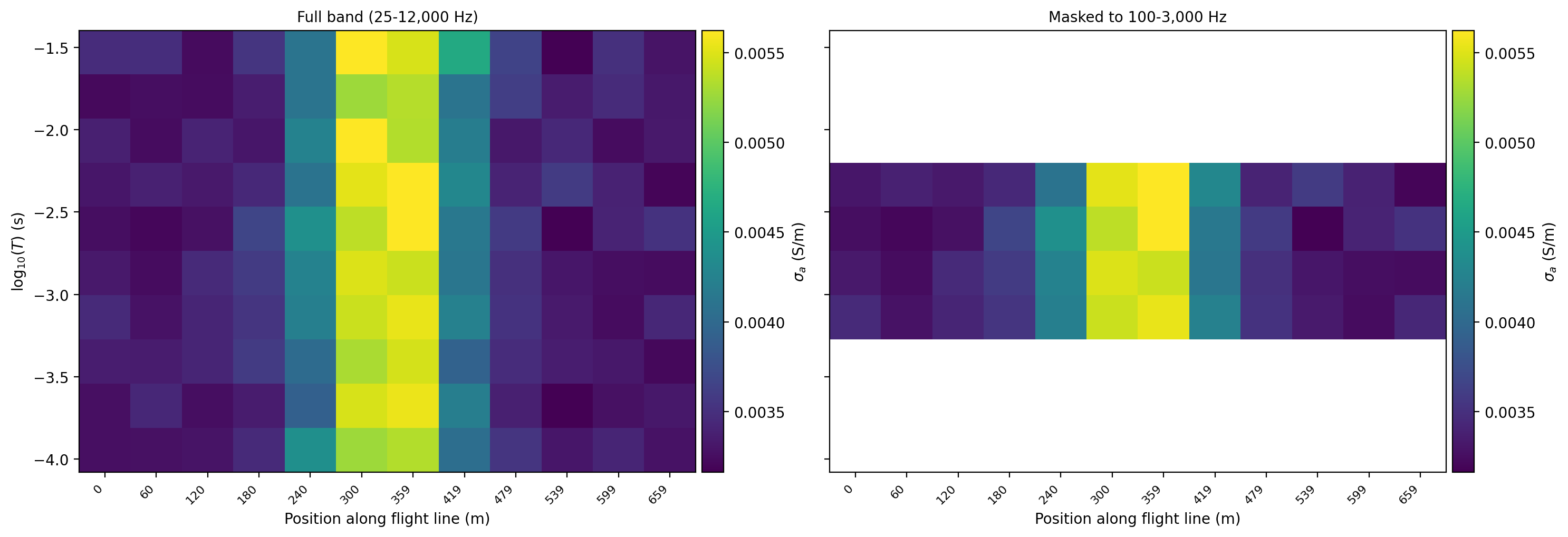
Native apparent conductivity, timiskaming_kimberlite_on: full
band (left) against masked to 100-3,000 Hz (right). Blank rows are
nan, not a fabricated zero.#
Masking never changes the frequency axis or drops a station – only
value cells go blank, exactly the three low and three high rows
numpy.ndarray.sum() counted above. This is deliberately
mask-only rather than drop-then-rebuild: each
AirborneEMRecord packages its admittance
tensor alongside auxiliary per-frequency fields (native apparent
conductivity, variance, covariances) around one shared period axis,
and safely dropping frequencies would require reconstructing all of
them consistently, which masking with nan avoids entirely.
Warning
Every file under data/mobileMT/ is synthetic, built by
inverting a simple resistivity-vs-position model into an admittance
tensor plus multiplicative noise – not a vendor delivery and
not a reproduction of either cited paper’s actual field data.
Each generated EMTF.description states this explicitly. No
proprietary MobileMT archive format is parsed anywhere in pyCSAMT;
pycsamt.airborne.mobilemt only maps already-decoded arrays
onto the common model.
11.16.5. Recommended Workflow#
The dropdown below reproduces every figure on this page end to end,
from the two ensure_mobilemt_dataset calls through the masked
pseudosection comparison:
View the executed workflow source codeClick to inspect and copy the complete code
1def run_emtools_mobilemt_workflow() -> None:
2    flammefjeld, timiskaming = _load_datasets()
3    make_admittance_profile(flammefjeld)
4    make_theoretical_vs_native(flammefjeld)
5    make_skew_profile(timiskaming)
6    make_band_mask_comparison(timiskaming)
11.16.6. References#
MobileMT’s physical model, the admittance-tensor formalism, and the co-located-sensor apparent-conductivity/skew derivations all follow [Prikhodko2022], [Sattel2019], and [Zhdanov2024]; see Airborne Natural-Source EM: AFMAG, ZTEM, And MobileMT for the full derivation shared with the other two airborne methods on this page’s predecessors, AFMAG Tilt-Angle Diagnostics And Motion-Coupling Physics and ZTEM Total-Divergence, Phase-Rotation, And Map-View Diagnostics. The skew ratio follows [Swift1967]’s original impedance-tensor formulation, applied here to the admittance tensor by direct algebraic analogy.