
7.5. Structural measurements#
StructuralMeasurement,
LinearMeasurement, and
FaultTrace record field structural evidence
against a profile position – the same role
Borehole plays for lithology, but for strike,
dip, and fault geometry instead of depth intervals.
StructuralModel collects all three per
profile. None of the four are electromagnetic, and none of them place
themselves anywhere except along the profile – see Package concepts
for why x is always a profile-relative metre value here, never a
latitude/longitude pair, and for how clone()/update()
re-validate an edited StructuralMeasurement (they do, because it
overrides validate(); not every class in this package does).
7.5.1. Recording a planar measurement#
A planar feature – bedding, foliation, a joint, a fault plane – is recorded as strike, dip, and dip direction, as a compass and clinometer would actually report it:
>>> from pycsamt.geology import StructuralMeasurement
>>> bedding = StructuralMeasurement(
...     x=500.0, kind="bedding",
...     strike_deg=45.0, dip_deg=30.0, dip_direction_deg=135.0,
... )
>>> bedding
StructuralMeasurement(x=500.0 m, 'bedding', 45/30->135)
kind is free text – 'bedding', 'foliation', 'joint',
'cleavage', 'contact', 'fault_plane', 'unconformity',
or a project-specific label – matching how
lithology is free text
rather than an enforced enumeration. strike_deg and
dip_direction_deg are compass bearings in [0, 360) degrees, not
reduced modulo 180: this module intentionally does not reuse MT
geoelectric strike’s axial (-90, 90] convention or the axial
mod-180 convention pycsamt.ai.geology.lenses uses for synthetic
ellipse geometry, because a raw compass reading is directed, not
axial, and reducing it early would throw that information away before
it can be cross-checked.
That cross-check is why dip_direction_deg is stored at all rather
than leaving strike to imply it through the right-hand rule:
dip_azimuth_ok requires
dip_direction_deg to sit within dip_direction_tolerance_deg
(20 degrees by default) of strike_deg + 90 or strike_deg - 90,
which catches a transposed field-notebook entry that recording only
one of the two numbers never would:
>>> bedding.dip_azimuth_ok
True
>>> StructuralMeasurement(
...     x=500.0, kind="bedding",
...     strike_deg=45.0, dip_deg=30.0, dip_direction_deg=200.0,
... )
Traceback (most recent call last):
    ...
ValueError: dip_direction_deg (200.0) is not within 20.0 deg of strike_deg (45.0) +/- 90 -- check for a transposed strike/dip-direction reading.
Drawing the strike line, the two acceptance wedges, and both the
accepted and rejected dip_direction_deg values on a compass rose
makes the geometry concrete:
View the strike/dip-direction geometry figure source codeClick to inspect and copy the complete code
 1def make_structural_measurement_geometry() -> None:
 2    """Write the strike/dip-direction compass diagram.
 3
 4    Shows the same ``bedding`` measurement used on the page (strike 45,
 5    dip direction 135, which ``dip_azimuth_ok``), the two +/-20 degree
 6    acceptance wedges centred on ``strike +/- 90`` that
 7    ``dip_direction_deg`` is checked against, and the rejected
 8    ``dip_direction_deg=200`` example that falls outside both wedges.
 9    """
10    bedding = StructuralMeasurement(
11        x=500.0, kind="bedding", strike_deg=45.0, dip_deg=30.0,
12        dip_direction_deg=135.0,
13    )
14    tol = bedding.dip_direction_tolerance_deg
15    strike = bedding.strike_deg
16    dipdir_ok = bedding.dip_direction_deg
17    dipdir_bad = 200.0
18
19    fig, ax = plt.subplots(figsize=(6, 6), subplot_kw={"projection": "polar"})
20    ax.set_theta_zero_location("N")
21    ax.set_theta_direction(-1)
22    ax.set_ylim(0, 1)
23    ax.set_yticklabels([])
24    ax.set_xticks(np.deg2rad([0, 90, 180, 270]))
25    ax.set_xticklabels(["N", "E", "S", "W"], fontsize=11)
26
27    for center in (strike + 90.0, strike - 90.0):
28        lo, hi = np.deg2rad(center - tol), np.deg2rad(center + tol)
29        theta = np.linspace(lo, hi, 30)
30        ax.fill_between(theta, 0, 1, color="#27AE60", alpha=0.18)
31
32    for ang in (strike, strike + 180.0):
33        ax.plot(
34            [np.deg2rad(ang), np.deg2rad(ang)], [0, 1],
35            color="#2C3E50", linewidth=2.5, solid_capstyle="round", zorder=3,
36        )
37
38    ax.annotate(
39        "", xy=(np.deg2rad(dipdir_ok), 0.92), xytext=(0, 0),
40        arrowprops=dict(arrowstyle="-|>", color="#1F618D", linewidth=2.5, mutation_scale=22),
41    )
42    ax.annotate(
43        "", xy=(np.deg2rad(dipdir_bad), 0.92), xytext=(0, 0),
44        arrowprops=dict(arrowstyle="-|>", color="#C0392B", linewidth=2.5, mutation_scale=22),
45    )
46
47    ax.text(np.deg2rad(dipdir_ok), 1.08, f"dip_direction_deg={dipdir_ok:.0f}\n(accepted)",
48            ha="center", va="center", fontsize=9, color="#1F618D")
49    ax.text(np.deg2rad(dipdir_bad), 1.15, f"dip_direction_deg={dipdir_bad:.0f}\n(rejected)",
50            ha="center", va="center", fontsize=9, color="#C0392B")
51    ax.text(np.deg2rad(strike) + 0.05, 0.55, f"strike_deg={strike:.0f}",
52            fontsize=9, color="#2C3E50")
53
54    ax.set_title(
55        "StructuralMeasurement geometry: strike, dip direction, and the\n"
56        "+/-20 deg acceptance wedges around strike +/- 90",
57        fontsize=11, pad=28,
58    )
59
60    fig.tight_layout()
61    fig.savefig(IMAGES / "structural_measurement_geometry.png", dpi=200, bbox_inches="tight")
62    plt.close(fig)
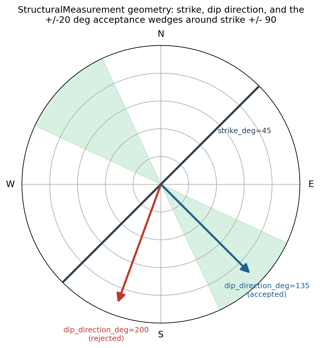
The black line is the strike (drawn both directions, since a strike
line has no single sense). The green wedges are the only
dip_direction_deg values dip_azimuth_ok accepts – 20 degrees
either side of strike +/- 90. 135 lands inside a wedge;
200 does not, which is exactly why the second construction above
raises.#
For anyone who prefers recording only dip direction and dip – the
common two-number field style –
from_right_hand_rule()
derives strike as dip_direction_deg - 90 under the right-hand-rule
convention (facing along strike, dip direction to your right), and
produces an identical, already-consistent measurement:
>>> rhr = StructuralMeasurement.from_right_hand_rule(
...     x=500.0, kind="bedding",
...     dip_direction_deg=135.0, dip_deg=30.0,
... )
>>> rhr.strike_deg == bedding.strike_deg
True
7.5.2. Recording a linear measurement#
A linear feature – a fold axis, a lineation, a slickenline – has no
dip direction to cross-check against, so
LinearMeasurement is simpler: just a
compass trend and a plunge below horizontal.
>>> from pycsamt.geology import LinearMeasurement
>>> fold_axis = LinearMeasurement(
...     x=500.0, kind="fold_axis", trend_deg=210.0, plunge_deg=15.0,
... )
>>> fold_axis
LinearMeasurement(x=500.0 m, 'fold_axis', 210/15)
7.5.3. Fault traces#
FaultTrace is coarser than the two leaf
measurements above – it is not a stereonet reading but a statement
about where a fault crosses this profile, which side dropped, and by
how much:
>>> from pycsamt.geology import FaultTrace
>>> fault = FaultTrace(
...     x=500.0, dip_deg=70.0, downthrown_side="right",
...     sense="normal", throw_m=12.0, evidence="resistivity offset",
... )
>>> fault
FaultTrace(x=500.0 m, dip=70 deg, down=right, throw=12.0 m)
dip_deg here is the apparent dip in the 2-D section, not
necessarily the fault’s true 3-D dip – the angle a single EM profile
can actually constrain, unless the line happens to run perpendicular
to strike. Pass the independently known strike_deg (from surface
mapping or a borehole) alongside it when the true attitude matters;
FaultTrace keeps the two separate rather than conflating them.
throw_m is always non-negative – direction is carried entirely by
downthrown_side, so a negative throw would be redundant with, and
could contradict, that field:
>>> FaultTrace(x=500.0, dip_deg=70.0, downthrown_side="right", throw_m=-5.0)
Traceback (most recent call last):
    ...
ValueError: throw_m (-5.0) must be >= 0; direction is carried by downthrown_side, not the sign of throw_m.
This is the class meant to plug into the structural-continuity
question Interpretation workflow already asks during misfit
review – “do apparent boundary offsets align with known structures?”
– with an actual record rather than an unbacked checklist item:
evidence names what supports the pick ('resistivity offset',
'borehole', 'surface mapping'), and sense
('normal', 'reverse', 'strike_slip', or the default
'unknown') records the kinematics where known.
7.5.4. Collecting evidence along a profile#
StructuralModel holds every planar
measurement, linear measurement, and fault trace for one profile
together:
>>> from pycsamt.geology import StructuralModel
>>> model = StructuralModel()
>>> model.add_planar(StructuralMeasurement(
...     x=200.0, kind="bedding",
...     strike_deg=40.0, dip_deg=25.0, dip_direction_deg=130.0,
... ))
>>> model.add_planar(StructuralMeasurement(
...     x=650.0, kind="bedding",
...     strike_deg=50.0, dip_deg=35.0, dip_direction_deg=140.0,
... ))
>>> model.add_fault(fault)
>>> model.add_fault(FaultTrace(
...     x=900.0, dip_deg=60.0, downthrown_side="left",
...     evidence="surface mapping",
... ))
>>> model
StructuralModel(2 planar, 0 linear, 2 faults)
Drawn as an actual cross section – fault traces tilted toward their
downthrown_side at their apparent dip_deg, bedding measurements
as strike/dip markers at the surface – this is the picture
StructuralModel is meant to back the structural-continuity review
mentioned above with:
View the structural evidence section figure source codeClick to inspect and copy the complete code
 1def make_structural_evidence_section() -> None:
 2    """Write the profile-section figure for a ``StructuralModel``.
 3
 4    Draws the two bedding measurements and two fault traces from the
 5    "Collecting evidence along a profile" example as an actual cross
 6    section: fault traces as dipping line segments (apparent dip,
 7    tilted toward ``downthrown_side``) and bedding measurements as
 8    triangular strike/dip markers at the surface.
 9    """
10    model = StructuralModel()
11    model.add_planar(StructuralMeasurement(
12        x=200.0, kind="bedding", strike_deg=40.0, dip_deg=25.0, dip_direction_deg=130.0,
13    ))
14    model.add_planar(StructuralMeasurement(
15        x=650.0, kind="bedding", strike_deg=50.0, dip_deg=35.0, dip_direction_deg=140.0,
16    ))
17    fault1 = FaultTrace(
18        x=500.0, dip_deg=70.0, downthrown_side="right", sense="normal",
19        throw_m=12.0, evidence="resistivity offset",
20    )
21    model.add_fault(fault1)
22    model.add_fault(FaultTrace(
23        x=900.0, dip_deg=60.0, downthrown_side="left", evidence="surface mapping",
24    ))
25
26    fig, ax = plt.subplots(figsize=(9, 5))
27
28    z_max = 80.0
29    for f in model.faults:
30        direction = 1.0 if f.downthrown_side == "right" else -1.0
31        z = np.array([0.0, z_max])
32        dx = direction * z / np.tan(np.deg2rad(f.dip_deg))
33        x_line = f.x + dx
34        color = _SENSE_COLOR[f.sense]
35        ax.plot(x_line, z, color=color, linewidth=2.5, zorder=3)
36        ax.annotate(
37            "down", xy=(x_line[1] + 25 * direction, z[1] * 0.35),
38            xytext=(x_line[1], z[1] * 0.35),
39            color=color, fontsize=8, va="center",
40            arrowprops=dict(arrowstyle="-|>", color=color, lw=1.2),
41        )
42        label = f"{f.sense}\ndip {f.dip_deg:.0f} deg"
43        if f.throw_m is not None:
44            label += f"\nthrow {f.throw_m:.0f} m"
45        ax.text(f.x, -6.0, label, ha="center", va="bottom", fontsize=8, color=color)
46
47    for m in model.planar:
48        ax.plot(m.x, 0.0, marker="v", color="#117864", markersize=10, zorder=4)
49        ax.text(
50            m.x, -6.0, f"{m.kind}\n{m.strike_deg:.0f}/{m.dip_deg:.0f}->{m.dip_direction_deg:.0f}",
51            ha="center", va="bottom", fontsize=8, color="#117864",
52        )
53
54    ax.set_xlim(0, 1050)
55    ax.set_ylim(z_max, -18)
56    ax.set_xlabel("Profile position x (m)")
57    ax.set_ylabel("Depth (m)")
58    ax.set_title("Structural evidence along the profile (StructuralModel)")
59    ax.grid(alpha=0.25)
60    ax.axhline(0.0, color="0.3", linewidth=0.8)
61
62    handles = [plt.Line2D([0], [0], color=c, lw=2.5, label=s) for s, c in _SENSE_COLOR.items()]
63    handles.append(plt.Line2D([0], [0], marker="v", color="#117864", linestyle="none",
64                              markersize=9, label="bedding measurement"))
65    ax.legend(handles=handles, loc="upper center", bbox_to_anchor=(0.5, -0.14),
66              fontsize=8, ncol=4, frameon=False)
67
68    fig.tight_layout()
69    fig.savefig(IMAGES / "structural_evidence_section.png", dpi=200, bbox_inches="tight")
70    plt.close(fig)
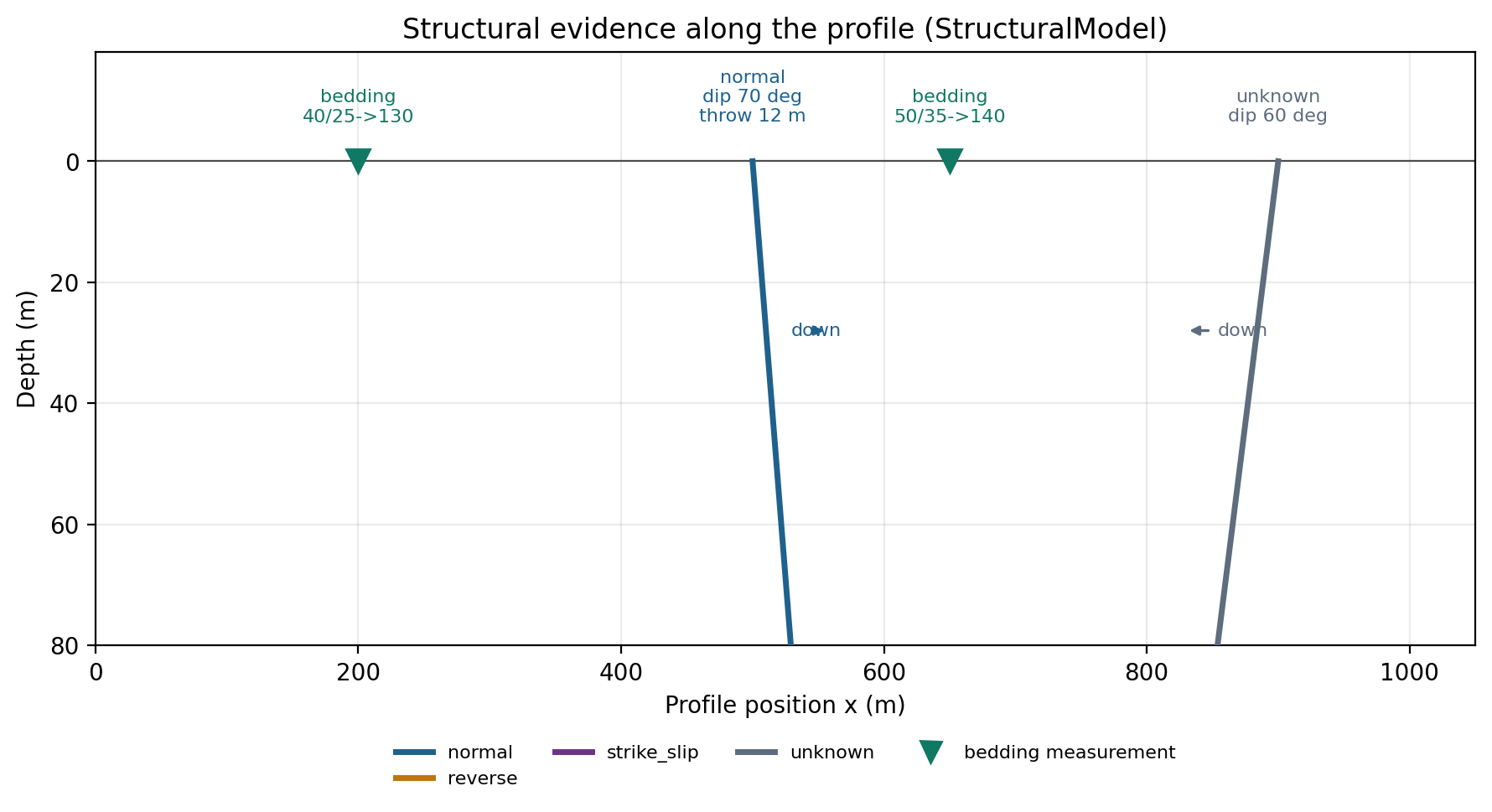
The normal fault at x=500 dips toward its downthrown (right)
side; the fault of unknown sense at x=900 dips toward its
downthrown (left) side. Both bedding markers sit at the surface
(z=None was not overridden), labelled with their recorded
strike/dip/dip-direction.#
within() restricts a model to a
profile span – useful for reviewing only the segment around one
inversion panel or station cluster – and returns a new
StructuralModel rather than mutating in place:
>>> model.within(0.0, 600.0)
StructuralModel(1 planar, 0 linear, 1 faults)
nearest() answers “what is the
closest piece of evidence of this kind to this position,” with an
optional max_distance so a distant match is not returned silently
as if it were locally relevant:
>>> model.nearest(520.0, kind="faults")
FaultTrace(x=500.0 m, dip=70 deg, down=right, throw=12.0 m)
>>> model.nearest(520.0, kind="faults", max_distance=5.0) is None
True
>>> model.nearest(300.0, kind="planar")
StructuralMeasurement(x=200.0 m, 'bedding', 40/25->130)
Like Borehole and
RockDatabase,
from_csv() loads field data
from disk – here, up to three independent CSV files, one per evidence
type, so a project can maintain separate spreadsheets for planar
readings, linear readings, and fault picks and combine only the ones
that exist:
x,dip_deg,downthrown_side,sense,throw_m,evidence
500.0,70.0,right,normal,12.0,resistivity offset
900.0,60.0,left,unknown,,surface mapping
>>> model_csv = StructuralModel.from_csv(faults_path="structure/faults.csv")
>>> model_csv
StructuralModel(0 planar, 0 linear, 2 faults)
>>> for f in model_csv.faults:
...     print(f)
FaultTrace(x=500.0 m, dip=70 deg, down=right, throw=12.0 m)
FaultTrace(x=900.0 m, dip=60 deg, down=left, throw=?)
The second row’s blank throw_m becomes None (unknown), not
zero – from_csv treats an empty field the same way
from_csv() and
from_csv() treat their own
optional columns elsewhere in this package. planar_path and
linear_path work the same way, with the column sets from
Recording a planar measurement and Recording a linear measurement
respectively; any path left as None simply yields an empty list
for that evidence type rather than an error.
7.5.5. Where to go next#
Interpretation workflow is where fault and structural evidence actually gets weighed against inversion results during misfit review. Rock resistivity database and Borehole logs cover the other two data families in this package.