
9.1. Basic Session#
A pycsamt.iot.FieldSession is the operational wrapper around an
IoT-enabled survey — the field session. It stores field devices,
station metadata, the accumulated telemetry packet stream,
monitoring thresholds, and the hand-off metadata that later processing can
audit. Everything else in this guide — edge QC, power budgeting,
clock synchronisation, provenance — ultimately reads from or writes into
one of these sessions, so it is the natural place to start.
The example below uses the repository’s real AMT demo line
data/AMT/WILLY_DATA/L18PLT to discover station identifiers from
EDI filenames. The live telemetry packets are synthetic because the
EDI files hold processed survey data, not an IoT packet stream. That split
is typical of this documentation: use real survey inventory where it
exists, and generate explicit, clearly labelled synthetic telemetry for the
acquisition layer that the EDI files do not carry.
9.1.1. Station Discovery#
Station IDs come from the first five EDI filenames on the L18 profile. In a field deployment the same IDs would usually come from the logger inventory or a station-occupation sheet rather than from processed files, but reusing real filenames here keeps the station identifiers grounded in an actual survey instead of an invented list.
>>> from pathlib import Path
>>> edi_dir = Path("data/AMT/WILLY_DATA/L18PLT")
>>> edi_files = sorted(edi_dir.glob("*.edi"))[:5]
>>> stations_from_data = [
...     path.stem.split("-")[-1].upper() for path in edi_files
... ]
>>> print(f"Real data path: {edi_dir.as_posix()}")
Real data path: data/AMT/WILLY_DATA/L18PLT
>>> print("Station ids:", ", ".join(stations_from_data))
Station ids: 001A, 002U, 003A, 004A, 005U
9.1.2. Devices And Stations#
Each station gets one recorder node. The station IDs and profile name come
from the real demo line; chainage, dipole geometry, and IoT device IDs are
deployment metadata supplied for the example. DeviceConfig
describes the physical recorder — protocol, sample rate, channels, role —
while StationConfig describes the field
occupation itself — position, dipole geometry, electrode azimuths, and the
device IDs attached to it. Keeping the two separate matters once a
deployment adds a remote-reference or gateway node that is not itself a
station occupation.
>>> from pycsamt.iot import DeviceConfig, StationConfig
>>> devices = []
>>> stations = []
>>> for index, (station_id, edi_file) in enumerate(
...     zip(stations_from_data, edi_files), start=1
... ):
...     device_id = f"l18-node-{index:02d}"
...     devices.append(
...         DeviceConfig(
...             device_id, station=station_id, protocol="file",
...             sample_rate_hz=512.0, channels=["ex", "ey", "hx", "hy"],
...             role="recorder",
...             metadata={
...                 "source_edi": edi_file.as_posix(),
...                 "source": "real L18PLT station id from repository data",
...             },
...         )
...     )
...     stations.append(
...         StationConfig(
...             station_id, profile="L18", position_m=(index - 1) * 50.0,
...             channels=["ex", "ey", "hx", "hy"], dipole_length_m=50.0,
...             ex_azimuth_deg=90.0, ey_azimuth_deg=0.0,
...             device_ids=[device_id],
...             notes=(
...                 "Station id taken from data/AMT/WILLY_DATA/L18PLT; "
...                 "IoT telemetry below is synthetic for documentation."
...             ),
...         )
...     )
>>> print((len(devices), len(stations)))
(5, 5)
9.1.3. Assembling The Session#
The FieldSession constructor accepts the
device and station lists directly; it is also where the monitoring
thresholds for this survey are declared. The
MonitoringConfig records the operational
expectations against which every future packet is judged: required
AMT channels, expected packet interval, maximum acceptable gap,
minimum battery voltage, maximum clock-offset, and the frequency band the
survey is meant to cover. Declaring these once at session creation, rather
than re-checking them ad hoc later, is what lets FieldSession.assess reduce an entire packet stream to
one status with a single call.
>>> from pycsamt.iot import FieldSession, MonitoringConfig
>>> session = FieldSession(
...     "WILLY-L18-IOT-DEMO", devices=devices, stations=stations,
...     method="amt", operator="pyCSAMT documentation",
...     monitoring_config=MonitoringConfig(
...         method="amt", expected_interval_s=60.0, max_gap_s=90.0,
...         min_packet_success_rate=0.95, min_edge_acceptance_rate=0.75,
...         min_battery_v=11.0, max_clock_offset_ms=5.0,
...         required_channels=["ex", "ey", "hx", "hy"],
...         frequency_band_hz=(1.0, 1000.0),
...     ),
...     metadata={
...         "real_data_path": edi_dir.as_posix(),
...         "telemetry_source": "synthetic QC packets for documentation",
...     },
... )
>>> print((session.survey_id, session.n_devices, session.n_stations, session.n_packets))
('WILLY-L18-IOT-DEMO', 5, 5, 0)
The session already knows about five devices and five stations because
add_device/add_station ran during construction, but n_packets is
still zero — a field session is populated with telemetry
packets incrementally as they arrive, not built from them up front.
9.1.4. Synthetic QC Telemetry#
The next block creates synthetic qc telemetry packets, three
per station. Four stations report accepted windows with a battery voltage
that decays gently across the profile and across packets, which is a
believable pattern for nodes that have been running for a while without a
fresh charge. The last station additionally reports one rejected window
with a low battery reading, so that the monitoring status below has
something concrete to flag.
>>> import numpy as np
>>> from pycsamt.iot import PacketKind, TelemetryPacket
>>> rng = np.random.default_rng(7)
>>> base_time = 1_700_000_000.0
>>> for index, (device, station) in enumerate(zip(devices, stations)):
...     for packet_index in range(3):
...         last_bad = (
...             station.station_id == stations[-1].station_id
...             and packet_index == 2
...         )
...         accepted = not last_bad
...         battery_v = (
...             10.7 if last_bad
...             else 12.6 - 0.12 * index - 0.03 * packet_index
...         )
...         payload = {
...             "method": "amt", "station": station.station_id,
...             "channels": ["ex", "ey", "hx", "hy"],
...             "frequency_band_hz": [1.0, 1000.0],
...             "accepted": accepted,
...             "decision": "accept" if accepted else "reject",
...             "battery_v": battery_v,
...             "clock_offset_ms": float(rng.normal(1.2, 0.35)),
...             "latency_s": float(rng.uniform(1.5, 4.5)),
...         }
...         _ = session.add_packet(
...             TelemetryPacket.from_device(
...                 device, timestamp=base_time + index * 180 + packet_index * 60,
...                 payload=payload, kind=PacketKind.QC,
...                 survey_id=session.survey_id,
...             )
...         )
>>> print(session.n_packets)
15
9.1.5. Session Tables And Status#
session.assess enriches each telemetry packet payload, then
reduces the stream to a monitoring status, and every quantity it
reports is reproducible outside pyCSAMT from the raw packet payloads shown
above. The packet success rate is the mean of the transport
acknowledgement flag \(a_i \in \{0, 1\}\) (ack_ok, true by default
when absent) over the \(N\) packets in the stream:
The edge acceptance rate only considers the subset of \(M \le
N\) packets that carry an edge quality control decision
\(d_j \in \{0, 1\}\) (accepted/decision in the payload):
so a stream with no edge decisions at all defaults to full acceptance rather than being penalised for missing metadata. Here \(N = M = 15\), so \(R_\mathrm{packet} = 1.0\) (every packet was acknowledged) and \(R_\mathrm{edge} = 14/15 \approx 0.933\) (one rejected window on the last station). The remaining status fields are order statistics over the packet timestamps \(t_i\), battery readings \(v_i\), and clock offsets \(c_i\):
with \(t_{(i)}\) the sorted timestamps. session.assess compares
these five quantities against the thresholds carried by the
MonitoringConfig declared above
(min_packet_success_rate, min_edge_acceptance_rate,
min_battery_v, max_clock_offset_ms,
max_gap_s/expected_interval_s), plus method and channel coverage
checks. Any violated threshold is recorded as an issue string, and the
overall monitoring status level is critical if the violated set
intersects a fixed critical subset (packet success, edge acceptance,
battery, clock offset, method mismatch, or missing required channels),
warning if other issues remain, and ok otherwise. The station,
packet, and status tables below make all of this concrete against the
fifteen packets just created:
>>> from pycsamt.iot import monitoring_status_table, packet_table
>>> station_df = session.station_table()
>>> print(
...     station_df[
...         ["station_id", "profile", "position_m", "channels", "device_ids"]
...     ].to_string(index=False)
... )
station_id profile  position_m    channels  device_ids
      001A     L18         0.0 ex;ey;hx;hy l18-node-01
      002U     L18        50.0 ex;ey;hx;hy l18-node-02
      003A     L18       100.0 ex;ey;hx;hy l18-node-03
      004A     L18       150.0 ex;ey;hx;hy l18-node-04
      005U     L18       200.0 ex;ey;hx;hy l18-node-05
>>> packet_df = packet_table(session.packets)
>>> print(
...     packet_df[
...         ["device_id", "kind", "timestamp", "payload_keys"]
...     ].head(5).to_string(index=False)
... )
  device_id kind    timestamp                                                                                    payload_keys
l18-node-01   qc 1700000000.0 accepted;battery_v;channels;clock_offset_ms;decision;frequency_band_hz;latency_s;method;station
l18-node-01   qc 1700000060.0 accepted;battery_v;channels;clock_offset_ms;decision;frequency_band_hz;latency_s;method;station
l18-node-01   qc 1700000120.0 accepted;battery_v;channels;clock_offset_ms;decision;frequency_band_hz;latency_s;method;station
l18-node-02   qc 1700000180.0 accepted;battery_v;channels;clock_offset_ms;decision;frequency_band_hz;latency_s;method;station
l18-node-02   qc 1700000240.0 accepted;battery_v;channels;clock_offset_ms;decision;frequency_band_hz;latency_s;method;station
>>> status = session.assess(now=base_time + 900.0)
>>> status_df = monitoring_status_table(status)
>>> print(
...     status_df[
...         ["level", "n_packet", "packet_success_rate",
...          "edge_acceptance_rate", "battery_min_v", "issues"]
...     ].to_string(index=False)
... )
   level  n_packet  packet_success_rate  edge_acceptance_rate  battery_min_v                  issues
critical        15                  1.0              0.933333           10.7 battery_below_threshold
The status lands on critical for a single reason: battery_min_v is
10.7, below the min_battery_v = 11.0 threshold declared earlier.
Note what did not trip the status — packet_success_rate is a perfect
1.0 and edge_acceptance_rate at 0.933 still clears the
configured min_edge_acceptance_rate = 0.75 comfortably. A stream can be
transported and QC-accepted almost perfectly and still be operationally
critical because one node’s power is failing; the level column and the
issues column answer two different questions and neither one can be
inferred from the other.
The pipeline hand-off reports a per-station acceptance rate rather than the stream-wide \(R_\mathrm{edge}\). For station \(s\) with \(n_\mathrm{accept}(s)\) accepted and \(n_\mathrm{reject}(s)\) rejected packets,
>>> pipeline = session.to_pipeline_input()
>>> for row in pipeline["stations"]:
...     print(
...         f"{row['station_id']}: n_packets={row['n_packets']}, "
...         f"acceptance_rate={row['acceptance_rate']:.2f}, "
...         f"band={row['accepted_band_hz']}"
...     )
001A: n_packets=3, acceptance_rate=1.00, band=[1.0, 1000.0]
002U: n_packets=3, acceptance_rate=1.00, band=[1.0, 1000.0]
003A: n_packets=3, acceptance_rate=1.00, band=[1.0, 1000.0]
004A: n_packets=3, acceptance_rate=1.00, band=[1.0, 1000.0]
005U: n_packets=3, acceptance_rate=0.67, band=[1.0, 1000.0]
which is why the first four stations report a clean 1.00 even though
the stream-wide \(R_\mathrm{edge}\) sits at 0.933 — the single
rejected packet belongs entirely to 005U, and \(R_\mathrm{edge}(s)\)
isolates it there instead of smearing it across the whole survey. A
downstream processing step that reads this hand-off can decide per station
whether 0.67 warrants a repeat occupation, without having to re-derive
that number from the raw packet stream itself.
9.1.6. The Field Dashboard#
session.station_table(), packet_table, and
monitoring_status_table are the tabular view of a session; the field
dashboard is the visual one. It gives a compact operational read of station
health, edge-QC acceptance, battery/synchronisation state, and
packet timing in a single figure, built entirely from the same
to_pipeline_input() data and
monitoring status computed above.
>>> from pathlib import Path
>>> from pycsamt.iot import plot_field_dashboard
>>> out_dir = Path("docs/source/images/user_guide/iot")
>>> out_dir.mkdir(parents=True, exist_ok=True)
>>> fig = plot_field_dashboard(
...     session, now=base_time + 900.0, station_axis="profile",
...     figsize=(10.8, 7.8),
...     output_path=(out_dir / "user-guide-iot-basic-session-01.png").as_posix(),
...     close=True,
... )
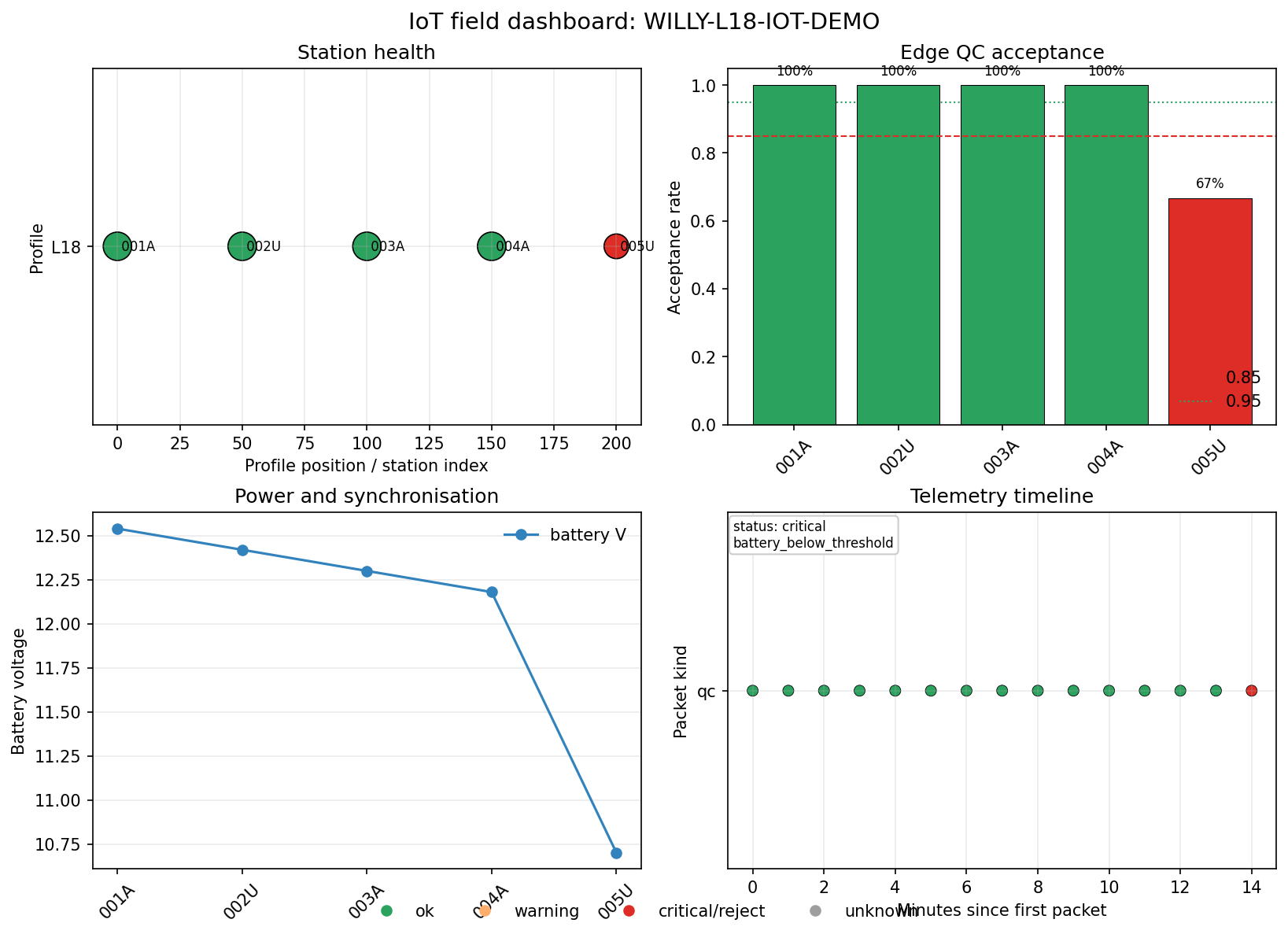
The field dashboard rendered from the fifteen QC packets above: station health along the profile (top left), edge QC acceptance per station (top right), battery and synchronisation trend (bottom left), and the telemetry timeline coloured by acceptance (bottom right).#
The top-left panel lays the five stations out along their profile chainage,
one marker per station, coloured by health_level and sized by
acceptance rate. Four markers sit green at 001A–004A; 005U
at chainage 200 m is red, the same conclusion the pipeline hand-off already
gave numerically. The top-right panel plots that same acceptance rate as a
bar per station against the two reference lines the plotting code draws at
0.85 and 0.95 — the first four bars clear both, 005U clears
neither, landing at 67%. The bottom-left panel is where the battery
decision surfaces visually: voltage declines steadily and almost linearly
across the profile — by construction, since each packet’s battery reading
was built as 12.6 - 0.12 * index - 0.03 * packet_index — and then drops
sharply to 10.7 V at 005U, well below the 11.0 V line that
alone accounts for the critical status. The bottom-right panel plots
all fifteen packets on a shared timeline spanning the fourteen minutes
between the first and last packet; every point is green except the very
last one, 005U’s third packet, which renders red for the same rejected
window already visible in the two panels above it. The status banner in
that panel — status: critical / battery_below_threshold — is the
one-line version of the whole figure.
9.1.7. Carrying Data Forward#
The station inventory in this example is grounded in the real L18 demo
dataset, while the telemetry is synthetic and explicitly marked as such.
That distinction matters: EDI files are downstream geophysical
products, but an IoT field session records the operational evidence
around acquisition, before any impedance has been computed. The
pipeline hand-off keeps those two layers connected by carrying
station IDs, channels, frequency-band coverage, packet counts, and
per-station acceptance rates forward into whatever processes the data
next — a report, a re-occupation decision, or eventually
FieldSession.to_edifiles
once real impedance is available. The next page,
Generic Edge QC, goes one level deeper: it works on the raw channel windows
before a packet like the ones above exists, and shows how the
accepted/decision fields this session already consumed are decided
in the first place.
9.1.8. Core Concepts#
DeviceConfigA recorder, gateway, remote-reference node, or sensor node. It stores protocol, sample rate, station assignment, channels, and role.
StationConfigA field occupation location. It stores coordinates, profile chainage, channel list, dipole geometry, orientation, operator, and attached devices.
TelemetryPacketA timestamped message with a canonical topic and payload. Packet kinds include
data,qc,health,sync,power,event, andsource(controlled-source transmitter telemetry).FieldSessionA stateful survey container that links devices, stations, packets, monitoring, station tables, pipeline inputs, and provenance manifests.
MethodProfileCanonical acquisition characteristics for an
EMMethod(AMT, MT, CSAMT, CSEM, TDEM/TEM): frequency band, required channels, nominal sample rate, and controlled-source / powerline-sensitivity flags. Profiles drive method-aware QC.
9.1.9. Scope Note#
The IoT layer records operational evidence around acquisition. It does not change the electromagnetic inversion itself. Edge packets can record finite-data coverage, spike and harmonic contamination indicators, frequency coverage, channel health, and accept/reject decisions. These metrics help identify poor acquisition windows and operational faults before downstream AMT/CSAMT processing, which is exactly what the fifth, red marker in the figure above was for.