
9.6. Bridging IoT Acquisition and the Data Model#
The IoT layer processes raw arrays and telemetry packets with
numpy only and stays independent of the heavier science API, which keeps
import pycsamt.iot cheap on a field gateway. The
pycsamt.iot.bridge module is the one place the two worlds meet.
Every science-API import (seg, site) is lazy, so pulling in the
bridge does not force the geospatial stack onto a node that only needs
telemetry.
The bridge works in both directions: forward, from edge impedance to the EDI/impedance tensor objects the processing flow expects, and in reverse, from an archived EDI survey back into a field session ready to re-occupy. The next three sections follow the forward direction end to end; the two after that follow it in reverse.
9.6.1. Impedance To Z#
The edge already forms per-window impedance estimates the same way
assess_impedance_stability() does for its
impedance stability check (see AMT/CSAMT Edge Diagnostics).
impedance_to_z() picks up from exactly that
point and turns the windows into a pycsamt.z.z.Z — the
impedance tensor container the processing and inversion flow
consumes — deriving an absolute error from the spread across windows. The
example below stands in for that edge output with a synthetic, noisy
half-space sounding on two L18 stations, so the whole page runs end to
end without a live acquisition:
>>> import numpy as np
>>> from pycsamt.iot import impedance_to_z, z_to_edi
>>> freq = np.logspace(4, 0, 12)              # 10 kHz -> 1 Hz, 12 points
>>> rng = np.random.default_rng(11)
>>> zxy_true = (1 + 1j) * np.sqrt(freq)        # flat rho_a, 45 deg phase
>>> z_windows = zxy_true[None, :] * (
...     1 + 0.03 * rng.standard_normal((6, freq.size))
... )                                          # 6 short synthetic edge windows
>>> z1 = impedance_to_z(z_windows, freq, station="18-001A", method="amt")
>>> print(f"Z tensor shape: {z1.z.shape}")
Z tensor shape: (12, 2, 2)
>>> print(f"Zxy[0] = {z1.z[0, 0, 1]:.3f}, Zyx[0] = {z1.z[0, 1, 0]:.3f}")
Zxy[0] = 99.808+99.808j, Zyx[0] = -99.808-99.808j
>>> rel_err = np.abs(z1.z_err[:, 0, 1]) / np.abs(z1.z[:, 0, 1])
>>> print(f"Median relative Zxy error: {np.median(rel_err):.3f}")
Median relative Zxy error: 0.022
That output is the whole aggregation rule made concrete. For a window
axis of size \(W\), impedance_to_z reduces the per-window scalar
estimates \(Z^{(w)}(f)\), \(w = 1, \dots, W\), to a mean (or,
with aggregate="median", a component-wise median) and reports the
spread across windows as an absolute error:
That is the same window-spread idea impedance stability uses to
score repeatability — here it becomes the z_err carried forward
instead of a pass/fail verdict. The default component="offdiag" then
places the aggregated scalar as an off-diagonal antisymmetry
pair, \(Z_{xy} = \bar{Z}\) and \(Z_{yx} = -\bar{Z}\), which is why
Zyx[0] above is exactly the negative of Zxy[0]. With six windows
and 3% per-window noise, the mean’s relative error settles around 2%,
matching the 0.022 printed above.
9.6.2. Z To EDI#
z_to_edi() (and the in-memory
build_edifile()) writes a preliminary EDI from
that tensor, so a field node can emit an .edi on site using the
station’s recorded geometry:
>>> from pathlib import Path
>>> path1 = z_to_edi(
...     z1, station="18-001A", lat=32.1203, lon=119.12883,
...     elevation=99.0, savepath="edi_out", method="amt",
... )
>>> print(f"Wrote: {Path(path1).name}")
Wrote: 18-001A.edi
When the optional geospatial stack is available,
z_to_site() returns a single EDI-backed
pycsamt.site.base.Site the same way, without needing a whole
session around it.
9.6.3. Session To EDI Files#
For a whole session, to_edifiles()
builds one EDI per station, enriched with the station geometry the
session recorded, and
to_sites_collection() promotes
the same impedance into a pycsamt.site.base.Sites collection
ready to feed straight to pycsamt.pipeline.Pipeline.run():
>>> from pycsamt.iot import FieldSession, StationConfig
>>> z2 = impedance_to_z(z_windows * 1.4, freq, station="18-002U", method="amt")
>>> session = FieldSession("L18-BRIDGE-DEMO", method="amt")
>>> _ = session.add_station(
...     StationConfig("18-001A", lat=32.1203, lon=119.12883, elevation=99.0)
... )
>>> _ = session.add_station(
...     StationConfig("18-002U", lat=32.1207, lon=119.12920, elevation=97.0)
... )
>>> edis = session.to_edifiles({"18-001A": z1, "18-002U": z2})
>>> for station_id, ed in edis.items():
...     print(f"  {station_id}: n_freq={ed.n_freq}, station={ed.station}")
  18-001A: n_freq=12, station=18-001A
  18-002U: n_freq=12, station=18-002U
>>> sites = session.to_sites_collection({"18-001A": z1, "18-002U": z2})
>>> print(f"Sites collection: {len(sites)} station(s)")
Sites collection: 2 station(s)
Station geometry travels with the impedance rather than being re-entered
by hand — to_edifiles looked up each station’s lat/lon/elevation from
the FieldSession itself. z2 reuses the same synthetic windows as
z1, scaled up by 1.4 in amplitude, purely so the figure below has two
visually distinct curves; nothing about that scaling is otherwise
meaningful.
A Z object already carries apparent resistivity and
phase — resistivity and
phase (and their _err
counterparts) are computed automatically from z/z_err by the
ResPhase base class the moment either is
set, using the practical-unit Cagniard convention
\(\rho_{a} = 0.2\,|Z|^2/f\). The figure below reads those attributes
directly rather than recomputing anything, and shows what actually ended
up inside the two EDIs: a flat apparent resistivity and a
constant 45-degree phase, the textbook signature of the
half-space sounding used to build z1/z2, with the per-window
spread from above carried through as error bars.
>>> import matplotlib.pyplot as plt
>>> out_dir = Path("docs/source/images/user_guide/iot")
>>> out_dir.mkdir(parents=True, exist_ok=True)
>>> fig, axes = plt.subplots(2, 1, figsize=(8.4, 6.4), sharex=True, constrained_layout=True)
>>> for z_obj, label, color in [(z1, "18-001A", "tab:blue"), (z2, "18-002U", "tab:orange")]:
...     _ = axes[0].errorbar(
...         1.0 / z_obj.freq, z_obj.res_xy, yerr=z_obj.res_err_xy,
...         marker="o", ms=4, color=color, label=label, capsize=2,
...     )
...     _ = axes[1].errorbar(
...         1.0 / z_obj.freq, z_obj.phase_xy, yerr=z_obj.phase_err_xy,
...         marker="o", ms=4, color=color, capsize=2,
...     )
>>> axes[0].set_xscale("log")
>>> axes[0].set_yscale("log")
>>> _ = axes[0].set_ylabel(r"$\rho_{a,xy}$ ($\Omega\cdot$m)")
>>> _ = axes[0].set_title("Edge impedance windows -> Z (impedance_to_z)")
>>> _ = axes[0].legend(loc="best")
>>> axes[0].grid(alpha=0.25, which="both")
>>> _ = axes[1].set_ylabel(r"$\varphi_{xy}$ (deg)")
>>> _ = axes[1].set_xlabel("Period (s)")
>>> axes[1].grid(alpha=0.25, which="both")
>>> fig.savefig(out_dir / "user-guide-iot-data-bridge-01.png", dpi=170)
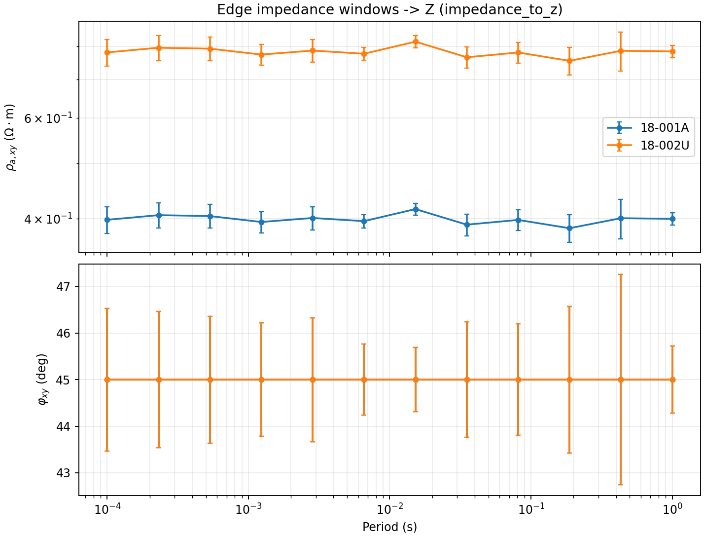
Both curves sit exactly where the construction predicts: 18-001A near
0.4 \(\Omega\cdot\)m and 18-002U near 0.78, a factor of
\(1.4^2 = 1.96\) apart since resistivity scales with \(|Z|^2\)
rather than \(|Z|\) — the amplitude bump used to separate the two
curves visually turns into a near-doubling of resistivity, not a 40%
change. The phase panel is flat at 45 degrees for both stations, because
zxy_true was built as \((1+i)\sqrt{f}\), and \(1+i\) has
exactly that angle at every frequency; only the error bars vary, growing
wider toward long period where fewer effective cycles went into each
window’s spectral estimate.
9.6.4. Consistent QC Via Emtools#
Field-side edge QC and downstream processing QC should not be two
independent notions of a “good” station.
emtools_qc() routes the sites the IoT layer
produced through the same coherence/skew/SNR quality control
the processing flow uses — see Quality-Control Confidence Scoring for the
confidence-ratio formulation behind these columns. Reusing the
session and impedance from above:
>>> from pycsamt.iot import emtools_qc
>>> table = emtools_qc(session, {"18-001A": z1, "18-002U": z2})
>>> flags = emtools_qc(session, {"18-001A": z1, "18-002U": z2}, flags=True)
>>> print(table[["station", "n_freq", "frac_ok", "snr_med"]].to_string(index=False))
station  n_freq  frac_ok   snr_med
18-001A      12      1.0 44.591203
18-002U      12      1.0 44.591203
>>> print(flags[["station", "frac_ok", "snr_med", "flags"]].to_string(index=False))
station  frac_ok   snr_med flags
18-001A      1.0 44.591203
18-002U      1.0 44.591203
Both stations come back clean here because the synthetic windows are
noise-free once aggregated and every row is finite — flags is empty
for both. A real edge deployment would carry error tensors down from
noisier windows and skewed diagonal terms from off-axis dipoles, which is
exactly what skew_med and the uncertainty/offdiag confidence
components pick up. emtools_qc also accepts an already-built
Sites collection or any EDI source, so the same QC can be re-run on
an archived survey later without touching the IoT layer at all.
Note
For a raw time series rather than pre-computed impedance, use
pycsamt.ts.ts_to_z() / pycsamt.ts.ts_to_edi(), which run
the spectral estimation for you. The bridge starts one step later,
from the impedance the edge has already estimated.
9.6.5. Seeding A Re-Occupation#
The bridge also reads an existing survey to plan a follow-up campaign.
Unlike the forward direction above, this side can run directly on the
repository’s real AMT demo line,
data/AMT/WILLY_DATA/L18PLT, rather than synthetic impedance —
field_session_from_edis() returns a
FieldSession with every station’s recorded
geometry and channels, plus a sensor node per station, ready to
re-occupy:
>>> from pycsamt.iot import field_session_from_edis, edi_survey_table
>>> edi_dir = "data/AMT/WILLY_DATA/L18PLT"
>>> reoccupy = field_session_from_edis(
...     edi_dir, survey_id="L18-REOCCUPY", method="amt", operator="crew"
... )
>>> print(f"stations={reoccupy.n_stations}, devices={reoccupy.n_devices}")
stations=28, devices=28
>>> device = list(reoccupy.devices.values())[0]
>>> print(f"first device: {device.device_id}, sample_rate_hz={device.sample_rate_hz:.1f}")
first device: 23-18-001A-node, sample_rate_hz=52000.0
>>> survey_tbl = edi_survey_table(edi_dir)
>>> print(
...     survey_tbl[
...         ["station", "lat", "lon", "n_freq", "f_min_hz", "f_max_hz"]
...     ].head(5).to_string(index=False)
... )
   station       lat        lon  n_freq  f_min_hz  f_max_hz
23-18-001A 32.120300 119.128833      53     1.008   10400.0
23-18-002U 32.121133 119.128900      53     1.008   10400.0
23-18-003A 32.122083 119.128850      53     1.008   10400.0
23-18-004A 32.123333 119.128833      53     1.008   10400.0
23-18-005U 32.123900 119.128833      53     1.008   10400.0
Every station on this line recovered the same 1.0–10400 Hz band, so the
seeded device’s sample_rate_hz is not read off the EDI — it is a
Nyquist-margin hint built from the highest recovered frequency,
which is why 52000.0 is exactly five times 10400.0 above. It is a
starting point for provisioning the re-occupying logger, not a recorded
acquisition parameter. The station geometry that seeds each new node is
the same lat/lon shown in the table, plotted below in profile order —
the line’s real layout, coloured by the same order the stations were
registered in:
>>> stations_ordered = list(reoccupy.stations.values())
>>> lats = [s.lat for s in stations_ordered]
>>> lons = [s.lon for s in stations_ordered]
>>> ids = [s.station_id for s in stations_ordered]
>>> fig2, ax2 = plt.subplots(figsize=(6.4, 8.2), constrained_layout=True)
>>> _ = ax2.plot(lons, lats, color="0.75", lw=1.0, zorder=1)
>>> sc = ax2.scatter(
...     lons, lats, c=np.arange(len(lons)), cmap="viridis", s=70,
...     zorder=2, edgecolor="none",
... )
>>> for idx in (0, 4, 8, 12, 16, 20, 24):
...     label = ids[idx].split("-")[-1]
...     _ = ax2.annotate(
...         label, (lons[idx], lats[idx]),
...         textcoords="offset points", xytext=(6, 4), fontsize=9,
...     )
>>> _ = ax2.set_xlabel("Longitude")
>>> _ = ax2.set_ylabel("Latitude")
>>> _ = ax2.set_title(f"L18PLT station geometry seeding the re-occupation ({len(ids)} stations)")
>>> _ = fig2.colorbar(sc, ax=ax2, label="Profile order")
>>> fig2.savefig(out_dir / "user-guide-iot-data-bridge-02.png", dpi=170)
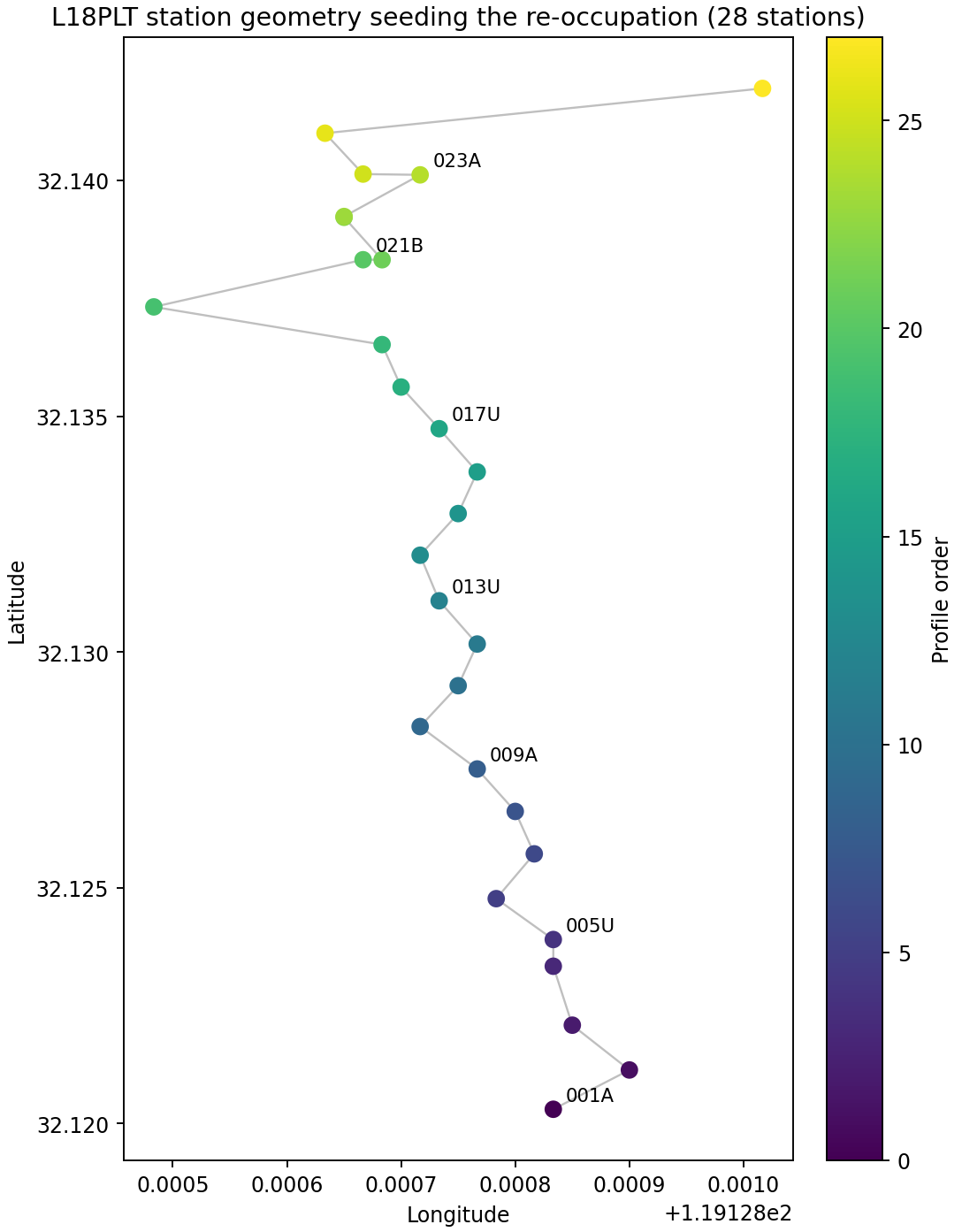
The line runs south to north from 001A up through 017U, 021B,
and 023A in mostly steady steps, but the colour bar exposes something
the raw geometry alone would not: stations 021B, 021U, 022U,
022V, 023A, and 023V (profile order 20–25) are all bunched
into the same small patch near the northern end, visibly closer together
than the rest of the line, before the final station 025A jumps well
to the east. That kind of infill is a deliberate acquisition choice —
denser sampling over a target of interest — and it is exactly the kind of
detail that is easy to miss reading station IDs in a table but obvious in
a profile-ordered map.
9.6.6. Deployment And Raw Records#
deployment_from_edis() is a lighter counterpart
that returns just a DeploymentConfig inventory, and
read_edi_survey() yields the raw per-station
summary records that both higher-level functions are built on:
>>> from pycsamt.iot import deployment_from_edis, read_edi_survey
>>> deployment = deployment_from_edis(
...     edi_dir, survey_id="L18-REOCCUPY", capabilities=["telemetry"]
... )
>>> print(f"deployment devices: {deployment.n_devices}")
deployment devices: 28
>>> records = read_edi_survey(edi_dir)
>>> print(f"read_edi_survey records: {len(records)}")
read_edi_survey records: 28
>>> print(records[0])
{'station': '23-18-001A', 'lat': 32.1203, 'lon': 119.12883333333333, 'elevation': 99.0, 'n_freq': 53, 'f_min_hz': 1.008, 'f_max_hz': 10400.0, 'channels': ['ex', 'ey', 'hx', 'hy']}
Sources may be a directory of .edi files, a glob pattern, a single
file or EDIFile, or any iterable mixing these — the same flexibility
read_edi_survey demonstrated above carries through to
field_session_from_edis, deployment_from_edis, and
emtools_qc.