
9.2. Generic Edge QC#
Generic edge diagnostics are the lightweight screening step that
can run on a field node before data are transmitted or stored. They are
not a replacement for AMT/CSAMT processing — they answer
simpler operational questions: is the window mostly finite, are there
obvious spikes, how many samples would be emitted after decimation,
and which edge decision should be attached to the packet? The
field session built in Basic Session already consumed
packets carrying exactly this accepted/decision pair; this page
shows where those fields come from.
The examples below use synthetic four-channel AMT-style windows.
That is appropriate here because generic edge QC works on live
time series arrays, not on EDI files — the decision has to
be made before a window is ever written to disk as processed data. Three
windows are created: a clean window, a marginal window with missing
Ey samples, and a bad window with missing electric and magnetic
samples plus spikes.
9.2.1. Synthetic Edge Windows#
Each row is a time series sample and each column is a channel, in
the order Ex, Ey, Hx, Hy. The marginal window drops one
channel over roughly 20% of the window and adds a short amplitude jump;
the bad window drops three channels over nearly a third of the window and
adds spikes on every twelfth Hy sample.
>>> import numpy as np
>>> sample_rate = 512.0
>>> n_samples = 2048
>>> t = np.arange(n_samples) / sample_rate
>>> rng = np.random.default_rng(31)
>>> channels = ["ex", "ey", "hx", "hy"]
>>> clean = np.column_stack(
...     [
...         np.sin(2 * np.pi * 7.0 * t) + 0.03 * rng.standard_normal(n_samples),
...         0.8 * np.sin(2 * np.pi * 9.0 * t + 0.2) + 0.03 * rng.standard_normal(n_samples),
...         0.3 * np.sin(2 * np.pi * 7.0 * t + 0.5) + 0.02 * rng.standard_normal(n_samples),
...         0.35 * np.sin(2 * np.pi * 9.0 * t + 0.8) + 0.02 * rng.standard_normal(n_samples),
...     ]
... )
>>> marginal = clean.copy()
>>> marginal[100:500, 1] = np.nan
>>> marginal[800:812, 0] += 4.0
>>> bad = clean.copy()
>>> bad[200:900, 0] = np.nan
>>> bad[260:880, 1] = np.nan
>>> bad[320:820, 2] = np.nan
>>> bad[::12, 3] += 10.0
>>> print((clean.shape, marginal.shape, bad.shape))
((2048, 4), (2048, 4), (2048, 4))
9.2.2. Coverage And Spike Detection#
EdgeProcessor decimates every fourth sample,
checks finite coverage, computes one channel summary per
channel, and estimates a robust spike fraction. With decimation
factor \(d\), pyCSAMT keeps samples \(0, d, 2d, \ldots\); for an
original window of \(N\) samples, the emitted count is
\(\lceil N/d \rceil\). After decimation, finite coverage is
A window below finite_threshold is rejected. A window above that hard
threshold but below warn_finite_threshold is accepted with a warning,
so data keeps flowing while the field audit trail still records that the
packet was marginal.
Spike detection is intentionally robust rather than mean/std-based. For each channel, the centre is the median \(m\), and the scale is \(1.4826\,\operatorname{median}(|x_i-m|)\), the usual normalised median absolute deviation. If that scale collapses to zero, pyCSAMT falls back to the standard deviation. A finite sample is counted as a spike when
where \(k\) is spike_threshold and \(s\) is the robust scale.
The channel spike fraction is the number of flagged finite samples divided
by the number of finite samples, and the window-level spike metric is the
maximum channel spike fraction — one badly behaved channel is enough to
flag the whole window, since a downstream transfer-function estimate would
be contaminated by it regardless of the other three channels’ health.
>>> from pycsamt.iot import EdgeProcessingConfig, EdgeProcessor
>>> processor = EdgeProcessor(
...     EdgeProcessingConfig(
...         decimation=4, finite_threshold=0.85, warn_finite_threshold=0.97,
...         channel_names=channels, spike_threshold=5.0,
...         max_spike_fraction=0.05, warn_spike_fraction=0.01,
...     )
... )
>>> results = [
...     processor.process(clean),
...     processor.process(marginal),
...     processor.process(bad),
... ]
>>> for label, result in zip(["clean", "marginal", "bad"], results):
...     warnings = result.metrics.get("warnings", "")
...     reasons = ";".join(result.reasons) or "-"
...     print(
...         f"{label}: decision={result.decision.value}, "
...         f"accepted={result.accepted}, "
...         f"finite={result.metrics['finite_coverage']:.3f}, "
...         f"max_spike={result.metrics['spike_fraction_max']:.3f}, "
...         f"warnings={warnings or '-'}, reasons={reasons}"
...     )
clean: decision=accept, accepted=True, finite=1.000, max_spike=0.000, warnings=-, reasons=-
marginal: decision=warning, accepted=True, finite=0.951, max_spike=0.000, warnings=finite_coverage_marginal, reasons=-
bad: decision=reject, accepted=False, finite=0.778, max_spike=0.334, warnings=-, reasons=finite_coverage_below_threshold;spike_fraction_above_threshold
The clean window’s 100% finite coverage is expected — nothing was removed
from it. The marginal window sits at 0.951, above finite_threshold but
still below the 0.97 warn line, so it is accepted with a warning rather
than silently passed. The bad window fails on two independent axes at
once: its 0.778 finite coverage is below the 0.85 hard threshold, and its
maximum channel spike fraction of 0.334 is far above max_spike_fraction
= 0.05 — either failure alone would have been enough to reject it.
9.2.3. Per-Channel QC#
edge_summary_table() unpacks the same three
results into one row per channel, which is where a window-level warning
or reject decision resolves into the specific channel actually
responsible. The result index identifies which edge window produced the
channel row: 0 is clean, 1 is marginal, 2 is bad.
>>> from pycsamt.iot import edge_summary_table
>>> summary = edge_summary_table(results)
>>> print(
...     summary[
...         [
...             "result_index", "channel", "finite_coverage",
...             "spike_fraction", "accepted", "decision", "reasons",
...         ]
...     ].to_string(index=False)
... )
 result_index channel  finite_coverage  spike_fraction  accepted decision                         reasons
            0      ex         1.000000        0.000000      True   accept
            0      ey         1.000000        0.000000      True   accept
            0      hx         1.000000        0.000000      True   accept
            0      hy         1.000000        0.000000      True   accept
            1      ex         1.000000        0.000000      True  warning
            1      ey         0.804688        0.000000     False  warning finite_coverage_below_threshold
            1      hx         1.000000        0.000000      True  warning
            1      hy         1.000000        0.000000      True  warning
            2      ex         0.658203        0.000000     False   reject finite_coverage_below_threshold
            2      ey         0.697266        0.000000     False   reject finite_coverage_below_threshold
            2      hx         0.755859        0.000000     False   reject finite_coverage_below_threshold
            2      hy         1.000000        0.333984     False   reject  spike_fraction_above_threshold
Marginal window 1 carries its warning decision on every channel
row, but only ey actually failed a per-channel threshold — its
0.804688 coverage is the one below finite_threshold = 0.85 that the
NaN block landed on. Bad window 2 shows the opposite pattern: three
channels (ex, ey, hx) fail on coverage because they were
zeroed out directly, while hy never lost a sample but still fails,
purely because the spikes injected every twelfth sample survived
decimation and pushed its spike fraction to 0.334.
9.2.4. Encode QC As Telemetry#
An EdgeProcessingResult can be converted
directly to a qc telemetry packet with
to_packet(). The packet
stores the compact metrics and all channel summaries, so a downstream
monitor can audit the edge decision without shipping the full waveform —
the same compact shape Basic Session built by hand is what this
method produces automatically from a real processing result.
>>> from pycsamt.iot import DeviceConfig, FieldSession
>>> device = DeviceConfig(
...     "l18-node-01", station="001A", protocol="file",
...     sample_rate_hz=sample_rate, channels=channels, role="recorder",
... )
>>> session = FieldSession("WILLY-L18-EDGE-QC", devices=[device], method="amt")
>>> base_time = 1_700_000_000.0
>>> for index, result in enumerate(results):
...     packet = result.to_packet(
...         device, timestamp=base_time + 60.0 * index,
...         survey_id=session.survey_id,
...     )
...     packet.payload.update(
...         {
...             "method": "amt", "station": "001A", "channels": channels,
...             "frequency_band_hz": [1.0, 1000.0],
...         }
...     )
...     _ = session.add_packet(packet)
>>> packet = session.packets[1]
>>> print(f"topic: {packet.topic}")
topic: pycsamt/WILLY-L18-EDGE-QC/001A/l18-node-01/qc
>>> print(f"decision: {packet.payload['decision']}")
decision: warning
>>> print(f"n channel summaries: {len(packet.payload['channels'])}")
n channel summaries: 4
>>> print(f"payload keys: {', '.join(sorted(packet.payload))}")
payload keys: accepted, channels, decision, frequency_band_hz, method, metrics, reasons, station
The packet pulled from index 1 is the marginal window, and its payload
carries decision: warning straight through — exactly the value the
window-level printout above already reported, now travelling with the
packet instead of living only in the local EdgeProcessingResult.
9.2.5. The Edge QC Figure#
plot_edge_qc_summary() turns the three results
into one diagnostic figure: decision counts, finite coverage per channel,
spike fraction per channel, and a tally of rejection reasons and warnings.
>>> from pathlib import Path
>>> from pycsamt.iot import plot_edge_qc_summary
>>> out_dir = Path("docs/source/images/user_guide/iot")
>>> out_dir.mkdir(parents=True, exist_ok=True)
>>> fig = plot_edge_qc_summary(
...     results, figsize=(10.8, 7.2), title="Synthetic edge QC windows",
...     output_path=(out_dir / "user-guide-iot-edge-qc-01.png").as_posix(),
...     close=True,
... )
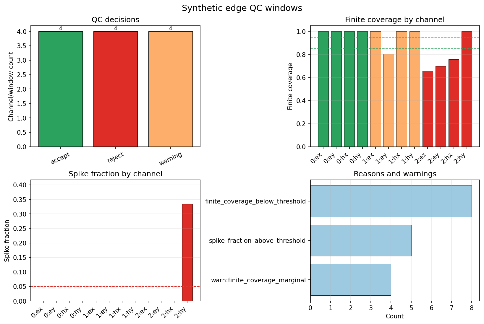
The edge QC figure built from the three synthetic windows: decision counts (top left), finite coverage per channel against the 0.85/0.97 thresholds (top right), spike fraction per channel against the 0.05 threshold (bottom left), and a tally of the reasons and warnings behind those decisions (bottom right).#
The top two panels are two views of the same twelve channel rows. The
decision-count bars show four channels each landed on accept,
warning, and reject — one window’s worth of channels apiece here,
though in general a single window can split its channels across
decisions. The finite-coverage panel colours every bar by that same
decision and draws the 0.85 and 0.97 lines the processor was configured
with, so 1:ey visibly sits in the warning band and all four 2:*
bars sit below the hard line. The spike-fraction panel is nearly empty by
design — only 2:hy clears the 0.05 threshold, which is exactly the
channel the synthetic spikes were injected into. The reasons panel counts
each window-level reason once per window and each channel-level reason
once per channel, rather than repeating a whole window’s reasons across
all of its channels: finite_coverage_below_threshold reaches 5 (the
bad window’s own window-level reason, plus 1:ey and the three failing
2:* channels), spike_fraction_above_threshold reaches 2 (the bad
window’s reason plus 2:hy), and warn:finite_coverage_marginal
reaches 1 — the marginal window’s single warning, counted once rather than
once per channel.
The clean window can be transmitted or stored as accepted telemetry
without further review. The marginal window is still usable at the window
level, but the ey channel coverage is low enough that the warning
belongs in the audit trail rather than being silently dropped. The bad
window fails both global finite coverage and spike-fraction thresholds, so
it should not be used for downstream transfer function or
impedance tensor work — generic edge QC caught that before any
AMT processing ever saw the window. Keep the thresholds themselves
in the deployment configuration or the provenance manifest, so a
survey reviewed later away from the instrument can reproduce exactly why
each window was accepted, warned, or rejected. The next page,
AMT/CSAMT Edge Diagnostics, builds on this generic layer with method-specific
checks — powerline harmonics, static shift, and impedance stability — that
only make sense once a window has already cleared the coverage and spike
screening shown here.