4.6. Boreholes in Map View

Map View can carry boreholes alongside a survey: as coloured tubes inside the 3-D section, as collar markers on the 2-D basemap, and as a side-by-side strip log. Every view derives from one canonical PCBH document — the single source of truth — so importing, editing, and exporting all round-trip through .pcbh.json.

4.6.1. Where the pieces live

Concern	Module / entry point
Format, validation, desurvey	pycsamt.format.borehole (read_pcbh, PCBHDocument)
Spreadsheet ingestion	pycsamt.format.borehole.inspect_workbook(), boreholes_from_xlsx()
Placing a hole in the 3-D scene	pycsamt.map.borehole_align.align_boreholes_to_scene()
Plotly figures (strip log, tubes, collars)	pycsamt.app._borehole (shared by the web and Map View apps)
The Map View UI	the Boreholes rail section and Borehole Studio modal

The worked example is the Baohuashan Cu–Mo AMT block. Kouabena et al. (2025, Ore Geology Reviews 185, 106798) drilled three holes on line L22 — ZK221, ZK222, ZK2203 — to confirm the mineralization predicted from the resistivity model. ZK2203’s 1101 m core record is in PAGEO-paper/geo/Lithgology and depth.xlsx; the three built, georeferenced holes and the reproducible build script are in PAGEO-paper/boreholes/ (see that folder’s README.md for full provenance — which parts are logged and which are digitized from the published figures).

4.6.2. Importing a field spreadsheet

Core logs rarely arrive tidy. inspect_workbook reports each sheet’s shape and its likely header rows without a bulk read:

>>> from pycsamt.format.borehole import inspect_workbook
>>> outline = inspect_workbook("PAGEO-paper/geo/Lithgology and depth.xlsx")
>>> for sheet in outline.sheets:
...     print(sheet.name, sheet.n_rows, sheet.n_cols,
...           sheet.header_candidates)
Lithgology and depth 176 17 [0, 1, 2, 3]
岩心牌 521 254 [0, 1, 2, 7, 9, 10, 11]

The Baohuashan ZK2203 workbook has a three-row merged header and a Rock name / Hole depth (m) From/To layout, and it carries no collar coordinates. Map the columns by index, supply the collar out of band, and import permissively:

>>> from pycsamt.format.borehole import boreholes_from_xlsx
>>> document, report = boreholes_from_xlsx(
...     "PAGEO-paper/geo/Lithgology and depth.xlsx",
...     sheet="Lithgology and depth",
...     header_row=3,
...     columns={"interval.lithology": 9,
...              "interval.from_md": 10,
...              "interval.to_md": 11},
...     constants={"borehole.id": "ZK2203"},
...     collars={"ZK2203": {"x": 700607.3, "y": 3556977.9,
...                          "z": 167.0, "crs": "EPSG:32650"}},
...     strict=False,
... )
>>> hole = document.boreholes[0]
>>> hole.id, hole.total_depth_md, len(hole.interval_logs["lithology"])
('ZK2203', 1100.52, 172)

report records every alias pick, the injected collar, and any rejected row. The result is a plain PCBHDocument — write it with write_pcbh. The paper’s build script PAGEO-paper/boreholes/build_boreholes.py does exactly this for all three L22 confirmation holes (ZK221, ZK222, ZK2203, drilled by Kouabena et al. 2025), attaching the ZK2203 core sample tags and the published Cu-Mo mineralization intervals, and writes PAGEO-paper/boreholes/baohuashan_l22.pcbh.json.

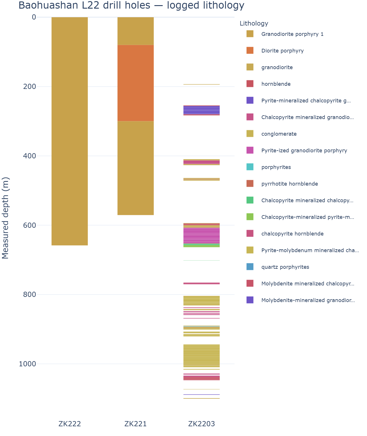
strip_log_figure(document) — the “linear” view of the three L22 holes. ZK2203 carries its full 172-interval core log (193–1101 m, real unlogged gaps preserved); ZK221 and ZK222 carry only the published host lithology (granodiorite porphyry 1, with a diorite-porphyry interval in ZK221).

A .xlsx whose header row already reads Rock name, From, To needs no columns= at all — the alias table resolves it, and a single-hole sheet only needs a collars= position.

4.6.3. Inserting a hole into the 3-D section

The 3-D volume builders (fence, block, iso-surface, depth-slice) do not work in easting/northing. They work in a local profile space: x along strike, y cross-strike, z elevation with depth downward from a topography datum. Dropping a collar’s real coordinates straight in would put it kilometres away.

pycsamt.map.geometry.survey_frame() fits the survey’s local frame (the same one the volume uses), and pycsamt.map.borehole_align.align_boreholes_to_scene() walks each desurveyed trajectory into it:

>>> from pycsamt.map import load_lines
>>> from pycsamt.map.geometry import survey_frame, survey_uv
>>> from pycsamt.map.borehole_align import (
...     align_boreholes_to_scene, surface_from_sections)
>>> from pycsamt.format.borehole import read_pcbh
>>> data = load_lines("PAGEO-paper/data/processed_edi",
...                    detect="folder", recursive=True)   # 128 stations
>>> document = read_pcbh(
...     "PAGEO-paper/boreholes/baohuashan_l22.pcbh.json")   # 3 holes
>>> ids = [s.id for s in data.stations]
>>> frame = survey_frame([s.latitude for s in data.stations],
...                      [s.longitude for s in data.stations],
...                      [s.line for s in data.stations])
>>> uv = survey_uv(ids, [s.latitude for s in data.stations],
...                [s.longitude for s in data.stations],
...                [s.line for s in data.stations])
>>> terrain = surface_from_sections([([uv[i][0] for i in ids],
...                                    [s.elevation for s in data.stations])])
>>> us = [uv[i][0] for i in ids]; vs = [uv[i][1] for i in ids]
>>> bounds = (min(us), max(us), min(vs), max(vs), -3000.0, 500.0)
>>> alignment = align_boreholes_to_scene(
...     document, frame, datum="surface", surface=terrain,
...     scene_bounds=bounds)
>>> {h.borehole_id: h.relation for h in alignment.placed}
{'ZK222': 'inside', 'ZK221': 'inside', 'ZK2203': 'inside'}

Each AlignedHole carries its centerline and vocabulary-coloured interval segments already in scene coordinates, plus an inside / edge / outside / unplaced relation and any datum warnings. pycsamt.app._borehole.scene_borehole_traces turns it into Mesh3d tubes (or fat poly-lines).

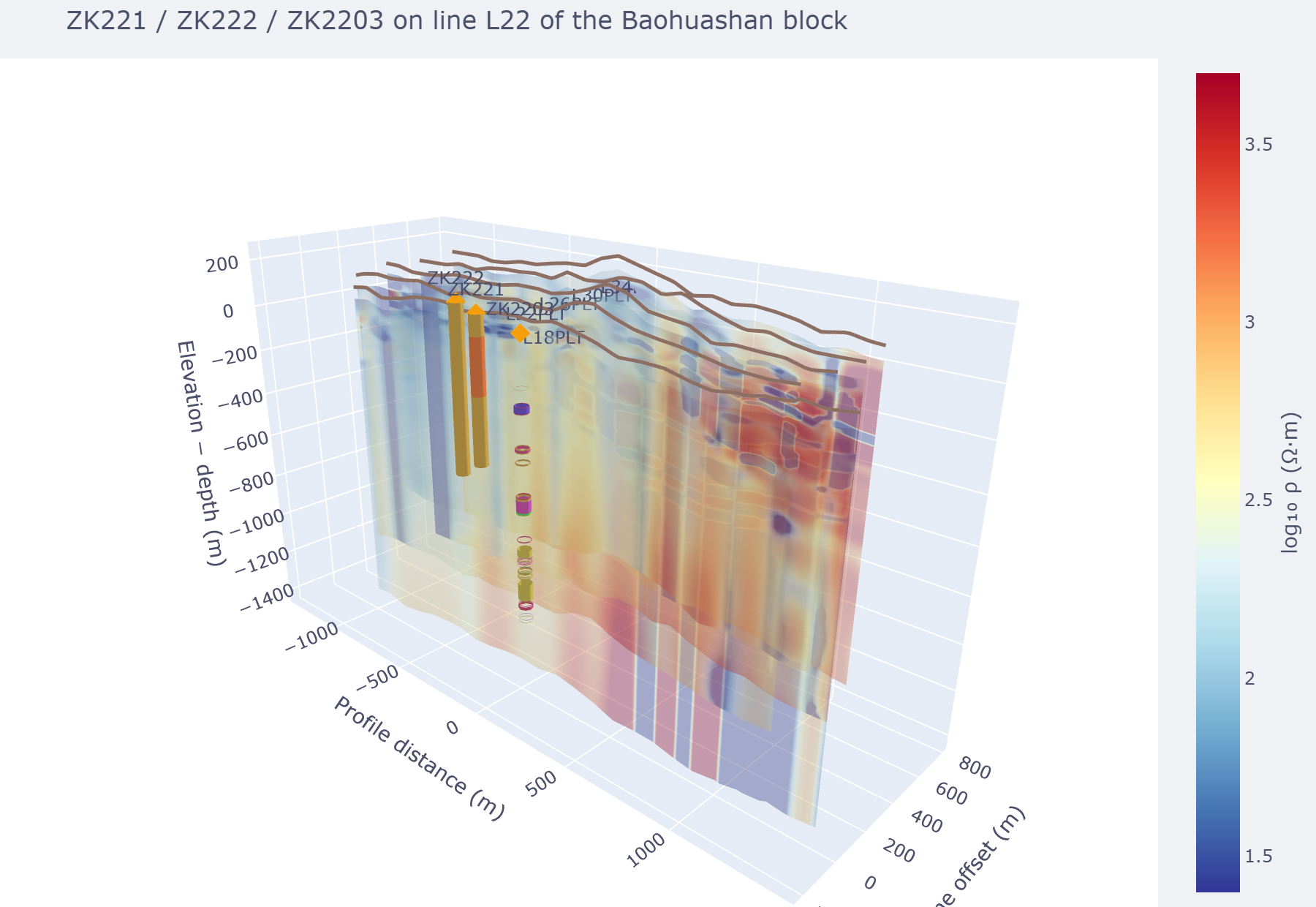
The three L22 confirmation holes on the Baohuashan fence section. Collars (digitized from Kouabena et al. 2025 Fig. 12b, ≈ stations 22-13 / 22-14 / 22-16) sit on the draped terrain line; the tubes descend through the imaged volume, clustered on the medium-resistivity anomaly they were drilled to test. ZK2203’s segmented column matches the strip log above.

4.6.4. The Borehole Studio

In Map View, the Boreholes rail button opens a workspace with a strip log / 3-D holes toggle, and Studio opens a modal with five tabs:

• Import — drop a .pcbh.json, a combined interval CSV, or an .xlsx (pick the sheet and header row, optionally type a x, y, z collar);

• Collars / Layers — editable tables, validated live against the PCBH schema, with a strip-log preview;

• Survey — a read-only desurvey preview (deviated trajectories enter via import);

• Preview — the strip log and the validation report.

The Import tab’s spreadsheet section also shows the sheet’s headers as Borehole id / Lithology / Depth from / Depth to dropdowns (auto-guessed by alias, overridable), so a merged multi-row header like the ZK2203 core sheet’s imports without touching a script.

Apply to view writes the document into the session. The hole then renders in the 3-D section, on the 2-D basemap, and in the Boreholes section. Export writes canonical .pcbh.json.

4.6.5. Targets and points of interest (PCPT)

Not every annotation is a logged hole. pycsamt.format.pointset adds a small .pcpt.json format for drill targets, planned collars, samples, and anomalies — a flat list of named positions, each with a location and an optional depth window. The paper’s baohuashan_l26_context.pcpt.json carries the previous L26 holes CK261, CK262 and the proposed location H01:

>>> from pycsamt.format import read_points
>>> l26 = read_points(
...     "PAGEO-paper/boreholes/baohuashan_l26_context.pcpt.json")
>>> [(p.id, p.kind) for p in l26.points]
[('CK262', 'sample'), ('CK261', 'sample'), ('H01', 'planned_borehole')]
>>> l26.lonlat()["H01"]
(32.127936, 119.124532)

points_from_csv and points_from_xlsx build the same object from a one-point-per-row table (id, lon/lat or x/y, optional depth_from / depth_to / kind / note).

The Studio’s Import tab has a Points / targets drop that accepts .pcpt.json, CSV, or .xlsx. Map View draws the points as kind-coloured markers on the 2-D basemap and as depth-stemmed markers in the 3-D scene, independent of any borehole, and the PCPT store travels in the session snapshot alongside the PCBH one.

Note

Reading .xlsx needs openpyxl (installed indirectly with pandas). The combined-CSV and spreadsheet importers share one assemble_interval_document core, so their reports, limits, and metre / ohm-metre unit requirement are identical.