4.7. MapView Session

pycsamt.map.MapView is the MapView session façade. It keeps one normalized MapData survey in memory and sends that same object to the station, profile, and volume renderers. This is useful when several views or exports must preserve exactly the same station order, line membership, coordinates, and source responses.

The session does not introduce a second plotting system. Its methods assemble the option dataclasses described in Station Maps, Profile Maps And Pseudosections, and 3-D Quick-Look Maps, then call their existing builders.

4.7.1. Create And Inspect A Session

For a directory containing one folder per line, use pycsamt.map.MapView.from_folder():

>>> from pycsamt.map import MapView

>>> mv = MapView.from_folder(
...     "data/AMT/WILLY_DATA",
...     detect="folder",
... )
>>> mv
MapView(lines=5, stations=128, geo=True)
>>> print(mv.lines)
('L18PLT', 'L22PLT', 'L26PLT', 'L30PLT', 'L34PLT')
>>> print(mv.stations[:5])
('18-001A', '18-002U', '18-003A', '18-004A', '18-005U')
>>> print(mv.n_stations, mv.has_geo)
128 True

detect="folder" applies pycsamt.map.load_lines() before the session is created. If line \(k\) contains \(N_k\) stations, the combined count is

(1)\[N = \sum_{k=1}^{K}N_k.\]

Here \(K=5\) and \(N=128\). The v2.1 ensure_sites behavior is applied while each line is normalized, including validated automatic chainage ordering. load_lines then re-indexes the combined records without losing their resolved line names.

An explicit mapping is preferable when scientific line names must not depend on directory names:

>>> selected = MapView.from_lines({
...     "north": "data/AMT/WILLY_DATA/L18PLT",
...     "south": "data/AMT/WILLY_DATA/L22PLT",
... })
>>> print(selected.lines, selected.n_stations)
('north', 'south') 53

The normalized station table is a convenient pre-flight record:

>>> table = mv.table()
>>> print(table.shape)
(128, 6)
>>> print(tuple(table.columns))
('ID', 'Latitude', 'Longitude', 'Elevation', 'Line', 'Index')
>>> table.groupby("Line").size().to_dict()
{'L18PLT': 28, 'L22PLT': 25, 'L26PLT': 25, 'L30PLT': 25, 'L34PLT': 25}

This table is derived from mv.data; editing it does not mutate the session.

4.7.2. Render Consistent Views

The convenience methods accept option fields directly as keyword overrides:

>>> station = mv.station(overlay="elevation", show_labels=False)
>>> pseudo = mv.pseudosection(
...     component="xy", by_line=True, line_cols=3
... )
>>> fence = mv.map3d(
...     mode="fence", depth_range=(0.0, 2000.0)
... )
>>> print("station traces:", len(station.data))
station traces: 10
>>> print("pseudosection panels:", len(pseudo.data))
pseudosection panels: 5
>>> print("3-D traces:", len(fence.data))
3-D traces: 15
>>> tuple(trace.type for trace in fence.data[:3])
('surface', 'scatter3d', 'scatter3d')

The ten station traces are five marker traces plus five profile lines. The pseudosection keeps the five traverses in separate panels; omitting by_line=True would concatenate unrelated lines onto one horizontal axis. The fence contributes three traces per line: a response curtain and supporting line/station geometry.

For elevation, elevation_mode makes the intended representation explicit. "markers" preserves the original station-colored view; "contours" interpolates a bounded elevation surface while retaining the acquisition tracks and station locations:

>>> elevation_contours = mv.station(
...     overlay="elevation",
...     elevation_mode="contours",
...     backend="matplotlib",
...     contour_mode="filled+lines",
...     contour_levels=16,
...     contour_interp="linear",
...     show_labels=True,
...     label_fontsize=5.2,
...     label_rotation=28.0,
... )
>>> print(
...     elevation_contours.axes[0].get_xlabel(),
...     elevation_contours.axes[0].get_ylabel(),
... )
Longitude Latitude

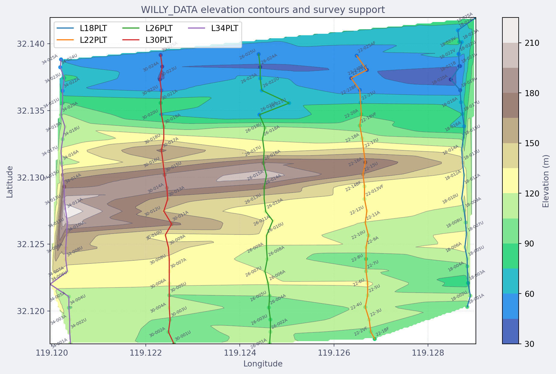
Elevation contours and line geometry from the shared 128-station session. Filled bands expose the broad north–south relief more clearly than isolated colors, while labeled station markers and five independently colored traverses show where that surface is supported. Linear interpolation is clipped to the observed elevation range; structure between widely separated lines remains an estimate.

</>View elevation-contour source codeClick to inspect and copy the complete code

def make_elevation_contour_map() -> None:
    """Render station elevations as contours while retaining field support."""
    view = MapView.from_folder(EDI, detect="folder", recursive=True)
    figure = view.station(
        options=StationMapOptions(
            backend="matplotlib",
            overlay="elevation",
            elevation_mode="contours",
            contour_mode="filled+lines",
            contour_levels=16,
            contour_opacity=0.82,
            contour_interp="linear",
            contour_smooth=0.5,
            contour_grid_res=220,
            cmap="terrain",
            marker_size=4,
            show_labels=True,
            label_fontsize=5.2,
            label_rotation=28.0,
            show_profiles=True,
            title="WILLY_DATA elevation contours and survey support",
        )
    )
    figure.set_size_inches(12.0, 7.4)
    axis = figure.axes[0]
    axis.grid(color="#94a3b8", linestyle=":", linewidth=0.65, alpha=0.5)
    axis.set_axisbelow(True)
    save_png(
        figure,
        IMAGES / "user-guide-map-mapview-01.png",
        dpi=190,
        bbox_inches="tight",
    )

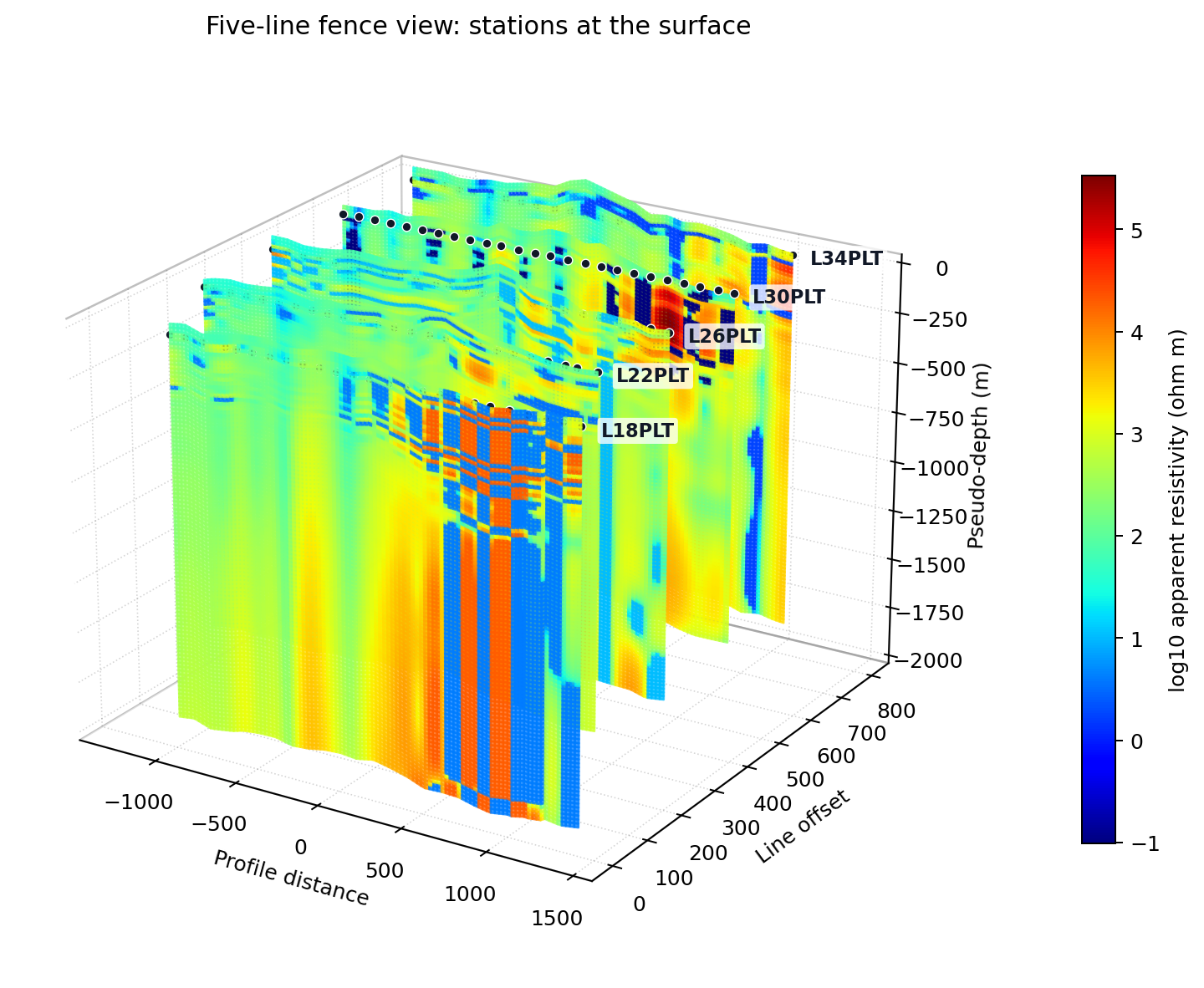
Fence curtains clipped to 2 km pseudo-depth. Their vertical coordinate is a skin-depth scale, not an inverted geological depth, so alignment between curtains is qualitative. Black markers locate the actual stations at z=0; line names sit beyond separate profile endpoints to avoid covering the data. Transparent panes and a light dotted grid keep depth reference lines visible without enclosing the curtains in a solid box.

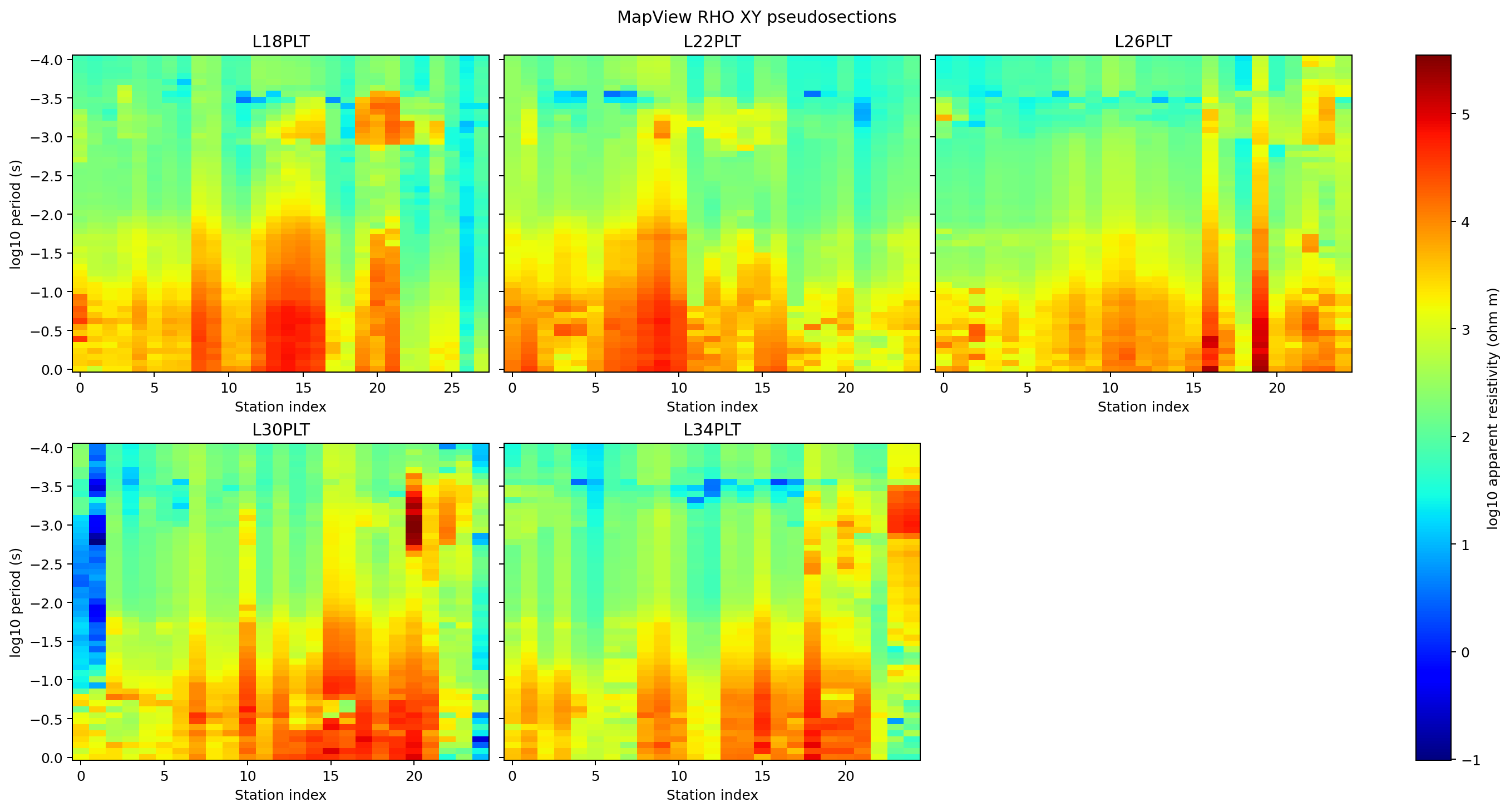
The same survey shown as five \(Z_{xy}\) apparent-resistivity pseudosections. A shared color scale supports cross-line comparison, while separate axes prevent false continuity between traverses.

For fence views, the approximate vertical scale used by the volume builder is

(2)\[\delta_{ik} \approx 503 \sqrt{\frac{\rho_{a,ik}}{f_k}} = 503\sqrt{\rho_{a,ik}T_k}\ \mathrm{m}.\]

Equation (2) is a penetration-depth estimate for an equivalent conductor. depth_range clips this derived coordinate; it does not constrain or solve an inversion.

4.7.3. Options, Defaults, And Overrides

The session-level theme and backend become defaults only when an options object is not supplied. Keyword overrides are applied last:

>>> from pycsamt.map import ProfileMapOptions

>>> dark = MapView(mv.data, theme="dark")
>>> options = ProfileMapOptions(
...     quantity="phase", components=("xy",), theme="publication"
... )
>>> phase = dark.pseudosection(options=options, x_axis="distance")
>>> print(phase.layout.title.text, phase.layout.xaxis.title.text)
PHASE XY pseudosection Distance (km)

Because options already specifies theme="publication", the session’s dark theme does not replace it. The direct x_axis override is then copied onto that options object without modifying the original.

4.7.4. Generic Figure Dispatch

Use pycsamt.map.MapView.figure() when the view name comes from a configuration file or interface control:

>>> fig = mv.figure(
...     "station", overlay="rho", frequency=10.0, show_labels=False
... )
>>> print(type(fig).__name__, len(fig.data))
Figure 10

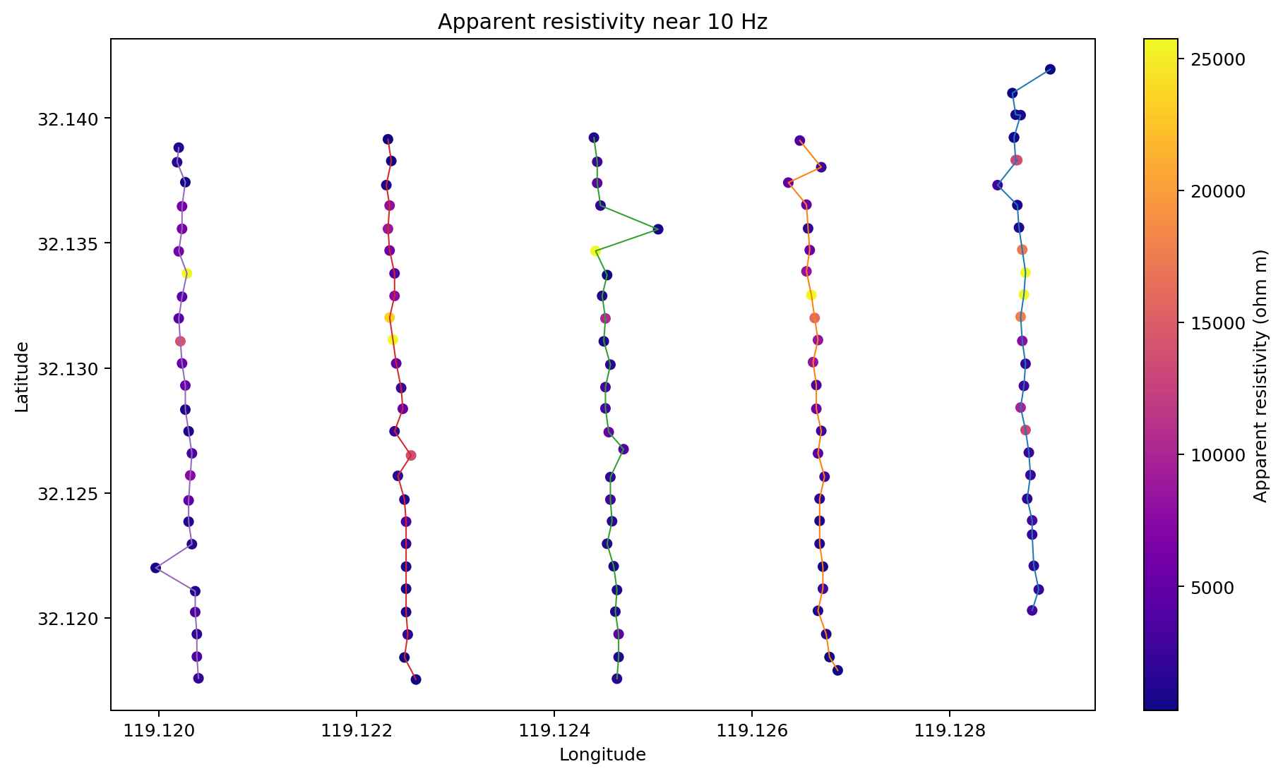
Apparent resistivity at the nearest recorded sample to 10 Hz. Color changes are measured station values; the connecting lines communicate acquisition geometry rather than interpolated resistivity.

Supported names are "station", "profile", "pseudosection", and "map3d". Unknown names fail explicitly:

>>> mv.figure("section")
Traceback (most recent call last):
...
ValueError: Unknown view 'section'. Expected one of ['map3d', 'profile', 'pseudosection', 'station'].

4.7.5. Elevation And Topography Handoffs

with_elevations returns a new session, which makes elevation corrections reproducible without changing the loaded survey:

>>> corrected = mv.with_elevations({"18-001A": 321.0})
>>> print(mv.data.stations[0].elevation)
99.0
>>> print(corrected.data.stations[0].elevation)
321.0
>>> print(corrected.n_stations)
128

Use export_topography to preserve station coordinates and elevations for a later inversion session. fetch_elevations performs an online lookup and should be treated as external data: archive its returned mapping and record the provider before applying it.

4.7.6. Export Reproducible Products

export renders one named view and delegates format handling to pycsamt.map.export_figure():

>>> path = mv.export(
...     "outputs/station.html",
...     view="station",
...     overlay="rho",
...     frequency=10.0,
... )
>>> print(path.as_posix())
outputs/station.html

export_all returns the paths keyed by view. Restricting views is useful when an expensive 3-D product is not required:

>>> written = mv.export_all(
...     "outputs/maps",
...     fmt="html",
...     views=("station", "pseudosection"),
... )
>>> {name: path.as_posix() for name, path in written.items()}
{'station': 'outputs/maps/station.html', 'pseudosection': 'outputs/maps/pseudosection.html'}

HTML contains the interactive Plotly specification and does not require Kaleido. Static Plotly image export does; see Exporting Map Figures.

4.7.7. Launch The Platform

mv.launch() hands this exact in-memory session to the optional Dash application. pycsamt.map.open_app() additionally accepts raw sources and constructs a session for them. GUI dependencies are optional, and launching starts a server, so it is deliberately not part of the reproducible non-interactive examples above. The application workflow is documented separately in MapView.