13.3. Location And Profiles

The site location tools handle station coordinates, topography assignment, coordinate projection, geodetic distance and bearing calculations, and survey-line chainage. The profile tools in pycsamt.site.profile build a 1-D profile line model from station locations so that a survey can be sorted, sliced, checked for gaps, and passed cleanly into processing or inversion preparation.

Use this page when you need to:

• parse latitude, longitude, or elevation values from field tables;

• normalize EDI HEAD coordinate fields;

• apply corrected GPS or topography tables to EDI sites;

• project lon/lat coordinates into another coordinate reference system;

• compute station spacing, bearing, or chainage along a survey line;

• infer the dominant line orientation from station coordinates;

• build a pycsamt.site.profile.Profile for line-ordered workflows.

The examples below use a small synthetic station class. It exposes the same get_section("head") pattern that pyCSAMT uses for EDI headers, so the outputs can be reproduced without depending on local EDI files.

>>> import copy
>>> import numpy as np

>>> class Head:
...     def __init__(self, name, lat=np.nan, lon=np.nan, elev=np.nan):
...         self.dataid = name
...         self.station = name
...         self.lat = lat
...         self.lon = lon
...         self.long = lon
...         self.elev = elev
...
>>> class DemoSite:
...     def __init__(self, name, lat=np.nan, lon=np.nan, elev=np.nan):
...         self.name = name
...         self.Head = Head(name, lat, lon, elev)
...
...     def get_section(self, key):
...         if str(key).lower() == "head":
...             return self.Head
...         return None
...
...     def set_section(self, key, value):
...         if str(key).lower() == "head":
...             self.Head = value
...
...     def __copy__(self):
...         new = type(self).__new__(type(self))
...         new.__dict__ = copy.deepcopy(self.__dict__)
...         return new
...
>>> def demo_sites():
...     return [
...         DemoSite("S01", 35.100, 12.700, 100.0),
...         DemoSite("S02", 35.105, 12.711, 105.0),
...         DemoSite("S03", 35.110, 12.722, 109.0),
...         DemoSite("S04", 35.125, 12.755, 120.0),
...     ]
...

13.3.1. Location Tool Map

Object or function	Scope	Main purpose
Coord	One coordinate.	Store latitude, longitude, and elevation as a small dataclass.
parse_lat(), parse_lon(), parse_elev()	Field values.	Parse decimal or DMS-like coordinate text into numeric values.
ensure_head_coords()	One EDI-like object.	Ensure the EDI HEAD section has numeric lat, lon/long, and elev fields.
apply_topography()	One or many sites.	Update site coordinates from a table matched by station identifier.
project()	Coordinate arrays.	Transform points between coordinate reference systems.
distance()	Two points.	Compute geodetic, flat, or projected distance in meters.
bearing()	Two points.	Compute azimuth from one point to another.
chainage_along()	One profile axis.	Project station positions onto a survey-line axis.

13.3.2. Profile Tool Map

Object or function	Main purpose
Profile	Store profile origin, azimuth, per-station chainage, spacing statistics, and detected large gaps.
Profile.from_sites()	Build a profile from EDI-like sites or Site wrappers.
Profile.sort_sites()	Return sites ordered by increasing chainage.
Profile.slice()	Return stations whose chainage lies inside a distance window.
Profile.resample()	Build a regular chainage grid between minimum and maximum station chainage.
Profile.summary()	Return spacing and gap summary statistics.
infer_line_orientation()	Estimate survey-line azimuth using PCA on local coordinate offsets.

13.3.3. Coordinate Containers

Use pycsamt.site.location.Coord when a small explicit coordinate object is clearer than passing loose tuples.

>>> from pycsamt.site.location import Coord

>>> station = Coord(lat=10.25, lon=20.75, elev=640.0)

>>> print(station.lat)
10.25
>>> print(station.lon)
20.75
>>> print(station.elev)
640.0

Coord does not validate values at construction time. Validation happens in helpers such as ensure_head_coords(), distance(), bearing(), and chainage_along().

13.3.4. Parsing Coordinates

Field coordinate tables are not always consistent. The parser accepts numeric values and common degree/minute/second style strings.

>>> from pycsamt.site.location import parse_elev, parse_lat, parse_lon

>>> lat1 = parse_lat("45N")
>>> lat2 = parse_lat("45 30 0 S")
>>> lon1 = parse_lon("123W")
>>> lon2 = parse_lon("123 15 30 E")
>>> elev = parse_elev("1200")

>>> print(lat1, lat2)
45.0 -45.5
>>> print(lon1, lon2)
-123.0 123.25833333333334
>>> print(elev)
1200.0

Parsing conventions:

• north and east are positive;

• south and west are negative;

• signed decimal values are accepted;

• unparseable values return NaN instead of raising;

• elevation is interpreted in meters.

Accepted examples include "10", "-3.2", "12 30 00 N", "12:30:00W", "3.5W", and numeric floats.

13.3.5. Normalizing EDI Head Coordinates

ensure_head_coords() creates or updates coordinate fields on an EDI-like object. It guarantees that the HEAD section carries numeric lat, lon, long, and elev values.

>>> from pycsamt.site.location import ensure_head_coords

>>> edi = DemoSite("S01")

>>> head = ensure_head_coords(
...     edi,
...     lat="35 07 30 N",
...     lon="12 45 00 E",
...     elev="1234",
... )

>>> print(head.lat, head.lon, head.long, head.elev)
35.125 12.75 12.75 1234.0

If a coordinate is missing or invalid, the function uses empty as the fallback sentinel. By default empty is 0.0.

For an invalid or absent coordinate, the sentinel is written explicitly:

>>> head = ensure_head_coords(
...     DemoSite("BAD"),
...     lat="bad",
...     lon=None,
...     elev=None,
...     empty=-9999.0,
... )
>>> print(head.lat, head.lon, head.elev)
-9999.0 -9999.0 -9999.0

Use this helper early when downstream code expects numeric coordinates.

13.3.6. Applying Topography Tables

apply_topography() updates one site, a list of sites, or a container with ._items from a table matched by station identifier.

>>> import pandas as pd

>>> from pycsamt.site.location import apply_topography

>>> collection = demo_sites()

>>> topo = pd.DataFrame(
...     {
...         "station": ["S01", "S02", "S03", "S04"],
...         "latitude": [35.100, 35.105, 35.110, 35.125],
...         "longitude": [12.700, 12.711, 12.722, 12.755],
...         "elevation": [101.0, 106.0, 110.0, 122.0],
...     }
... )

>>> updated = apply_topography(collection, topo, inplace=False)
>>> for site in updated:
...     print(site.name, site.Head.lat, site.Head.lon, site.Head.elev)
...
S01 35.1 12.7 101.0
S02 35.105 12.711 106.0
S03 35.11 12.722 110.0
S04 35.125 12.755 122.0

Station identifiers are matched case-insensitively against common columns: station, site, dataid, id, and name. Coordinate columns are searched among:

Coordinate	Accepted columns
Latitude	latitude, lat.
Longitude	longitude, lon, long.
Elevation	elevation, elev, alt.

Use inplace=False when you want a copied structure and inplace=True when the input objects should be updated directly.

13.3.7. Coordinate Projection

project() transforms coordinate pairs between coordinate reference systems. When pyproj is available, pyCSAMT uses it with always_xy=True. GDAL is used as a fallback when available.

>>> from pycsamt.site.location import project

>>> x, y = project(
...     [(12.5, 35.25), (12.6, 35.30)],
...     crs_from="EPSG:4326",
...     crs_to="EPSG:32633",
... )

>>> print(np.round(x, 2))
[272542.59 281776.97]
>>> print(np.round(y, 2))
[3903632.75 3908954.73]

Important convention: projected coordinate pairs are interpreted as (x, y). For geographic CRS values, that means (lon, lat) when using EPSG:4326 with this function. Keeping this order explicit is important for reproducibility because the same two numbers swapped as (lat, lon) project to a different place.

If neither pyproj nor GDAL is available, project() raises RuntimeError.

13.3.8. Distance And Bearing

distance() computes the distance between two coordinates in meters. Three modes are available:

mode="geodetic"

Haversine approximation on a spherical Earth. This is the default.

mode="flat"

Local small-extent planar approximation using latitude-scaled longitude distances.

mode="utm"

Project both points to UTM, or to crs_to when supplied, and compute Euclidean distance.

>>> from pycsamt.site.location import Coord, bearing, distance

>>> a = Coord(0.0, 0.0, 0.0)
>>> b = Coord(0.0, 1.0, 0.0)

>>> d = distance(a, b, mode="geodetic")
>>> az = bearing(a, b)

>>> print(d)   # about 111 km at the equator
111194.92664455874
>>> print(az)  # about 90 degrees, east
90.0

bearing() uses the same mode names. It returns azimuth in degrees with 0 degrees pointing north and 90 degrees pointing east.

The geodetic distance is based on:

(1)\[d = 2R \arcsin \left( \sqrt{ \sin^2(\Delta \phi / 2) + \cos \phi_1 \cos \phi_2 \sin^2(\Delta \lambda / 2) } \right).\]

The geodetic bearing uses the spherical forward azimuth:

(2)\[\theta = \operatorname{atan2} \left( \sin\Delta\lambda \cos\phi_2,\, \cos\phi_1 \sin\phi_2 - \sin\phi_1 \cos\phi_2 \cos\Delta\lambda \right).\]

Equation (1) returns surface separation, whereas equation (2) returns the direction of travel from the first coordinate to the second; reversing the points therefore changes the bearing and does not generally produce the same angle plus exactly 180 degrees on a sphere.

13.3.9. Chainage Along A Line

chainage_along() projects station coordinates onto a survey-line axis. The axis is defined by an origin and azimuth. Azimuth follows the geophysical line convention used in pyCSAMT: 0 degrees is north and 90 degrees is east.

>>> from pycsamt.site.location import chainage_along

>>> origin = (0.0, 0.0)
>>> station = (0.0, 1.0 / 111.0)  # about 1 km east near the equator

>>> s = chainage_along(origin, azimuth=90.0, pts=station)
>>> print(s)
1000.0

For local offsets \(dx\) east and \(dy\) north, chainage is:

(3)\[s = dx \sin A + dy \cos A,\]

where \(A\) is the profile azimuth in radians.

Equation (3) is a signed projection, not cumulative distance between successive stations. A station can therefore have a small chainage even when it lies far from the line if most of its displacement is cross-track.

The function returns a scalar for one point and a NumPy array for a sequence of points.

>>> points = [
...     (0.0, 0.0),
...     (0.0, 1.0 / 111.0),
...     (0.0, 2.0 / 111.0),
... ]

>>> chainages = chainage_along(origin, 90.0, points)
>>> print(chainages)
[   0. 1000. 2000.]

13.3.10. Inferring Line Orientation

infer_line_orientation() estimates the dominant survey-line axis from a set of site coordinates. It builds local Cartesian offsets and applies PCA. The principal component with the largest variance defines the line direction.

>>> from pycsamt.site.profile import infer_line_orientation

>>> collection = demo_sites()
>>> azimuth = infer_line_orientation(collection)
>>> print(round(azimuth, 1))
60.9

The returned azimuth is in degrees, with 0 degrees north and 90 degrees east. Because a line axis has no intrinsic direction, the result should be interpreted modulo 180 degrees. For example, 45 degrees and 225 degrees describe the same line axis.

Mathematically, pyCSAMT first converts station coordinates to local offsets \(x\) east and \(y\) north about the mean station position:

(4)\[x_i = (\lambda_i-\bar{\lambda})\,M\cos\bar{\phi}, \qquad y_i = (\phi_i-\bar{\phi})\,M,\]

where \(M\) is the metres-per-degree scale, \(\lambda\) is longitude, and \(\phi\) is latitude. PCA then finds the unit vector \(\mathbf{v}=(v_x,v_y)\) with maximum projected variance. The profile azimuth is the north-clockwise angle of that vector, \(A=\operatorname{atan2}(v_x,v_y)\). The local scaling in equation (4) prevents raw longitude degrees from being treated as the same physical length as latitude degrees away from the equator.

13.3.11. Ordering Sites Along A Survey Line

File discovery order, station-name order, and physical profile order are different concepts. pycsamt.site.base.Sites.ordered() makes that choice explicit without renaming stations or changing their data. It accepts six primary modes:

by	Ordering key	Appropriate use
"input"	Preserve the current container order.	Replaying acquisition or a deliberately prepared manifest. Directory enumeration is not automatically a meaningful input order.
"station"	Natural numeric station name, so S2 precedes S10.	Lines whose identifiers were assigned monotonically during acquisition.
"latitude"	Increasing latitude; missing coordinates are placed last.	Predominantly north–south lines known to progress northward.
"longitude"	Increasing longitude; missing coordinates are placed last.	Predominantly east–west lines known to progress eastward.
"chainage"	Projection onto the PCA line axis.	Forcing spatial order when the caller has already established that the coordinates represent a profile.
"auto"	Chainage only after geometry checks; otherwise input order.	The safest general default for unknown survey geometry.

The distinction is visible in the bundled 25-station L22PLT line. The example deliberately begins with case-insensitive lexical filenames, which put 22-013VF and 22-025AF before 22-10U and therefore do not describe acquisition progress:

>>> from pathlib import Path
>>> from pycsamt.seg.edi import EDIFile
>>> from pycsamt.site.base import Sites

>>> data_dir = Path("data/AMT/WILLY_DATA/L22PLT")
>>> paths = sorted(data_dir.glob("*.edi"), key=lambda path: path.name.casefold())
>>> l22 = Sites([EDIFile(path) for path in paths])

>>> for mode in ("input", "station", "latitude", "longitude", "chainage", "auto"):
...     ordered_l22 = l22.ordered(mode)
...     print(
...         mode,
...         ordered_l22[0].name,
...         ordered_l22[-1].name,
...         ordered_l22.ordering["applied"],
...     )
...
input 22-013VF 22-9A input
station 22-1BF 22-025AF station
latitude 22-1BF 22-025AF latitude
longitude 22-23VF 22-1BF longitude
chainage 22-1BF 22-025AF chainage
auto 22-1BF 22-025AF chainage

auto does not merely alias chainage. It converts valid coordinates to local east/north offsets, fits the PCA axis, and evaluates

(5)\[L=\frac{\sigma_1^2}{\sigma_1^2+\sigma_2^2}, \qquad C=\frac{\operatorname{range}(u_\perp)} {\operatorname{range}(u_\parallel)}, \qquad F=\frac{N_{\mathrm{finite}}}{N_{\mathrm{sites}}},\]

where \(L\) is profile linearity, \(C\) is the cross-track ratio, and \(F\) is the finite-coordinate fraction. Automatic chainage is applied only when these quantities meet the configured thresholds. The ordering report records both the requested and applied modes so downstream code can audit the decision:

>>> report = l22.ordered("auto").ordering
>>> print(report["applied"])
chainage
>>> print(round(report["linearity"], 5))
0.99994
>>> print(round(report["cross_track_ratio"], 4))
0.0136
>>> print(round(report["span_m"], 1), round(report["azimuth"], 1))
2353.4 359.4

The line is therefore almost due north, more than 99.99% of its coordinate variance lies along one axis, and its full cross-line spread is only about 1.36% of its along-line span. Those numbers justify the automatic decision; they are more informative than the word chainage alone.

The following plot uses color for returned position and a grey segment between successive sites. It displays the same coordinates in every panel, so only the ordering rule changes:

>>> import matplotlib.pyplot as plt
>>> import numpy as np

>>> coords = np.asarray([site.coords[:2] for site in l22], dtype=float)
>>> lat0, lon0 = np.mean(coords, axis=0)

>>> def local_offsets(ordered_sites):
...     ll = np.asarray([site.coords[:2] for site in ordered_sites], dtype=float)
...     east = (ll[:, 1] - lon0) * 111_000.0 * np.cos(np.radians(lat0))
...     north = (ll[:, 0] - lat0) * 111_000.0
...     return east, north
...
>>> modes = ("input", "station", "latitude", "longitude", "chainage", "auto")
>>> fig, axes = plt.subplots(2, 3, figsize=(11, 8), constrained_layout=True)
>>> for axis, mode in zip(axes.ravel(), modes):
...     ordered_l22 = l22.ordered(mode)
...     east, north = local_offsets(ordered_l22)
...     rank = np.arange(1, len(ordered_l22) + 1)
...     _ = axis.plot(east, north, color="0.75", linewidth=1.0)
...     points = axis.scatter(
...         east, north, c=rank, cmap="viridis", s=34,
...         edgecolor="black", linewidth=0.35, zorder=2,
...     )
...     _ = axis.annotate("1", (east[0], north[0]), xytext=(5, 3),
...                       textcoords="offset points", fontsize=8, weight="bold")
...     _ = axis.annotate("25", (east[-1], north[-1]), xytext=(5, 3),
...                       textcoords="offset points", fontsize=8, weight="bold")
...     applied = ordered_l22.ordering["applied"]
...     _ = axis.set_title(f"by={mode!r}  →  {applied}")
...     _ = axis.set_xlabel("cross-line east offset (m)")
...     _ = axis.set_ylabel("north offset (m)")
...     axis.grid(True, alpha=0.22)
...     axis.set_box_aspect(1)
...
>>> colorbar = fig.colorbar(points, ax=axes, shrink=0.82, pad=0.02)
>>> colorbar.set_label("position in returned order")
>>> _ = fig.suptitle("L22PLT: all Sites.ordered modes")
>>> fig.savefig("location_profile_l22_ordering.png", dpi=180)

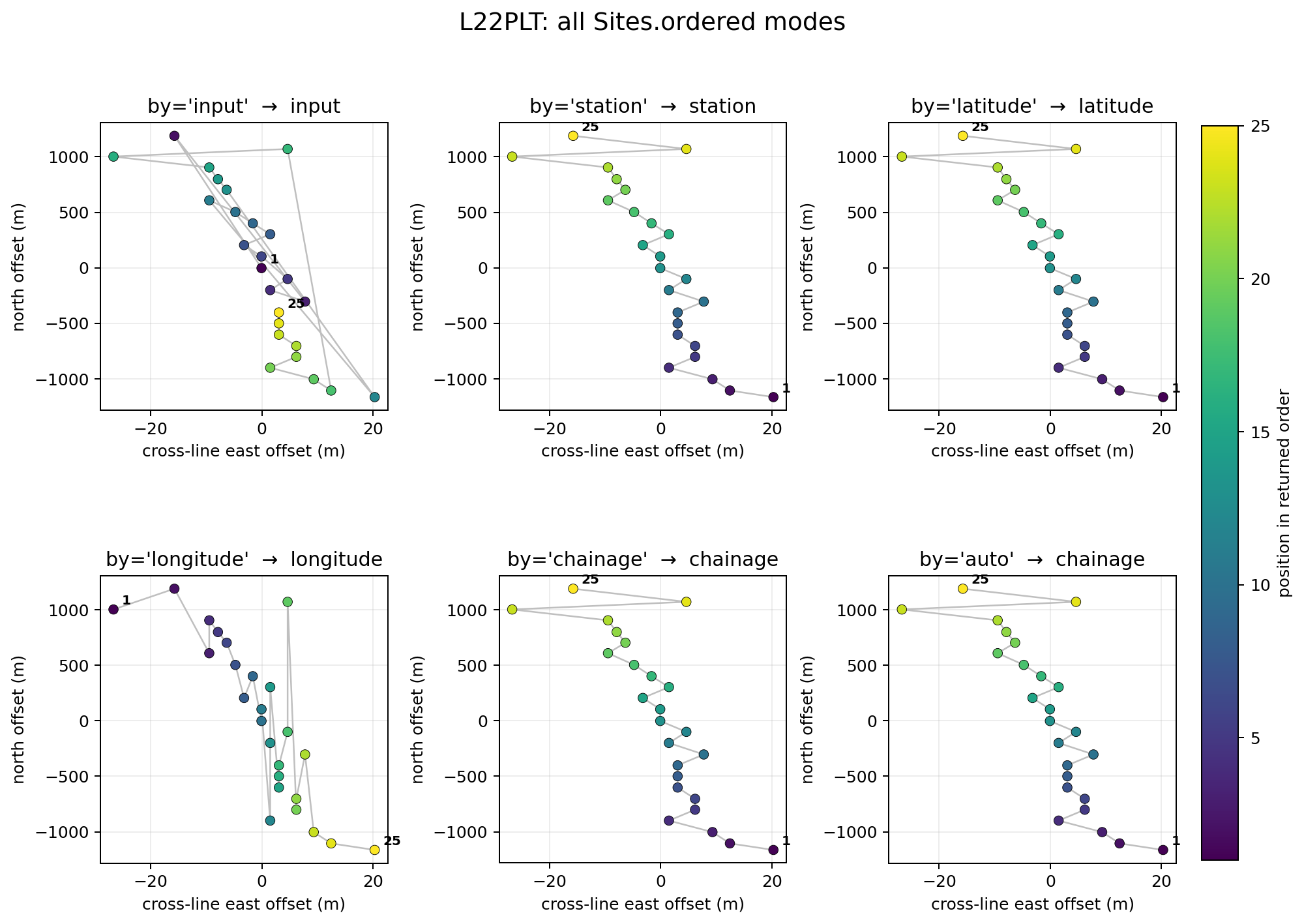
The same L22PLT coordinates under every supported ordering mode. Dark purple is the first returned site and yellow is the last; grey connections reveal jumps between consecutive sites.

The input panel crosses the line repeatedly because lexical filenames are not a profile coordinate. longitude is also unsuitable here: the line is north–south, so sorting on its small east–west GPS deviations produces a sequence that moves backward and forward along the line. Natural station and latitude happen to agree with chainage for this survey, but that is a property of L22PLT, not a general guarantee. auto reaches the same result as forced chainage only after validating the geometry.

Missing coordinates are another important difference. Forced chainage keeps such sites at the end in their original relative order, preserving the container membership for later repair. By contrast, Profile.sort_sites() drops sites without a finite chainage because a profile cannot place them along its axis. Choose between those behaviors deliberately rather than treating both operations as interchangeable.

13.3.12. Building Profiles

Profile stores a survey-line representation:

• origin as a pycsamt.site.location.Coord;

• azimuth in degrees;

• chainages as {station_name: chainage_m};

• spacing_stats for line spacing;

• gaps for large station-spacing intervals.

Build one from sites:

>>> from pycsamt.site.profile import Profile

>>> collection = demo_sites()
>>> profile = Profile.from_sites(collection)

>>> print(round(profile.azimuth, 1))
60.9
>>> print({k: round(v, 1) for k, v in profile.chainages.items()})
{'S01': 0.0, 'S02': 1142.8, 'S03': 2285.6, 'S04': 5713.9}
>>> print({k: round(v, 1) for k, v in profile.spacing_stats.items()})
{'spacing_mean': 1904.6, 'spacing_med': 1142.8, 'spacing_min': 1142.8, 'spacing_max': 3428.3}
>>> print([(round(a, 1), round(b, 1)) for a, b in profile.gaps])
[(2285.6, 5713.9)]

If no origin is supplied, the first finite site coordinate is used. If no azimuth is supplied, infer_line_orientation() is used.

>>> import matplotlib.pyplot as plt
>>> import numpy as np

>>> lons = np.array([site.Head.lon for site in collection])
>>> lats = np.array([site.Head.lat for site in collection])
>>> names = [site.name for site in collection]
>>> chainage = np.array([profile.chainages[name] for name in names])
>>> elev = np.array([site.Head.elev for site in collection])

>>> fig, ax = plt.subplots(1, 2, figsize=(8, 3.4), constrained_layout=True)
>>> _ = ax[0].plot(lons, lats, marker="o")
>>> for lon, lat, name in zip(lons, lats, names):
...     _ = ax[0].annotate(
...         name, (lon, lat), textcoords="offset points", xytext=(4, 4)
...     )
...
>>> _ = ax[0].set_xlabel("longitude")
>>> _ = ax[0].set_ylabel("latitude")
>>> _ = ax[0].set_title("Station map")
>>> ax[0].margins(0.08)

>>> _ = ax[1].plot(chainage, elev, marker="s")
>>> for s, z, name in zip(chainage, elev, names):
...     _ = ax[1].annotate(
...         name, (s, z), textcoords="offset points", xytext=(4, 4)
...     )
...
>>> for left, right in profile.gaps:
...     _ = ax[1].axvspan(left, right, alpha=0.15)
...
>>> _ = ax[1].set_xlabel("chainage (m)")
>>> _ = ax[1].set_ylabel("elevation (m)")
>>> _ = ax[1].set_title("Profile chainage")
>>> ax[1].margins(0.08)

>>> for axis in ax:
...     axis.grid(True, alpha=0.25)
...
>>> fig.savefig("location_profile_chainage.png", dpi=160)

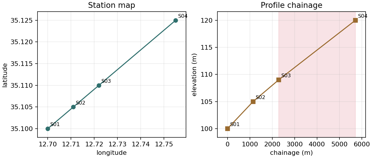
The same four stations shown geographically and as a line profile. The shaded interval marks the large chainage gap detected by the profile summary rule.

You can also force both:

>>> from pycsamt.site.location import Coord

>>> custom_profile = Profile.from_sites(
...     collection,
...     origin=Coord(35.0, 12.0, 0.0),
...     azimuth=90.0,
... )

For the synthetic line, forcing an east-directed profile from the first station gives simple east-west chainages:

>>> east_profile = Profile.from_sites(
...     collection,
...     origin=Coord(35.1, 12.7, 0.0),
...     azimuth=90.0,
... )
>>> print({k: round(v, 1) for k, v in east_profile.chainages.items()})
{'S01': 0.0, 'S02': 999.0, 'S03': 1997.9, 'S04': 4994.8}

13.3.13. Sorting And Slicing Profiles

Use Profile.sort_sites() to return sites ordered by increasing chainage. Sites without finite coordinates are dropped.

>>> ordered = profile.sort_sites(collection)
>>> print([site.name for site in ordered if hasattr(site, "name")])
['S01', 'S02', 'S03', 'S04']

Use Profile.slice() to select a chainage window:

>>> window = profile.slice(500.0, 2500.0)
>>> print({k: round(v, 1) for k, v in window.items()})
{'S02': 1142.8, 'S03': 2285.6}

The returned mapping is ordered by chainage.

13.3.14. Resampling And Summary

Profile.resample() builds a regular chainage grid between the minimum and maximum station chainage.

>>> grid = profile.resample(step=250.0)
>>> print(np.round(grid, 1).tolist())
[0.0, 250.0, 500.0, 750.0, 1000.0, 1250.0, 1500.0, 1750.0, 2000.0, 2250.0, 2500.0, 2750.0, 3000.0, 3250.0, 3500.0, 3750.0, 4000.0, 4250.0, 4500.0, 4750.0, 5000.0, 5250.0, 5500.0]

Profile.summary() returns spacing and gap information:

>>> summary = profile.summary()

>>> print(summary["n_sites"])
4.0
>>> print(round(summary.get("spacing_mean"), 1))
1904.6
>>> print(round(summary.get("spacing_med"), 1))
1142.8
>>> print(summary["n_gaps"])
1.0

Spacing statistics include:

Key	Meaning
spacing_mean	Mean station spacing in meters.
spacing_med	Median station spacing in meters.
spacing_min	Minimum station spacing in meters.
spacing_max	Maximum station spacing in meters.
s_min, s_max	Minimum and maximum finite chainage.
n_sites	Number of stations with finite chainage.
n_gaps	Number of large spacing gaps.

13.3.15. Gap Detection

After chainages are sorted, Profile computes station spacings with numpy.diff. A large gap is recorded when spacing exceeds 1.5 * median_spacing. Gaps are stored as (s_left, s_right) chainage intervals.

>>> if profile.gaps:
...     for left, right in profile.gaps:
...         print(f"Gap from {left:.1f} m to {right:.1f} m")
...
Gap from 2285.6 m to 5713.9 m

This is a simple QC rule, not a geological interpretation. Use it to find survey-line acquisition holes, missing stations, or irregular spacing before building inversions or pseudo-sections.

13.3.16. End-To-End Example

The following example applies a topography table, builds a profile, sorts the survey, and checks spacing.

>>> import pandas as pd

>>> from pycsamt.site.location import apply_topography
>>> from pycsamt.site.profile import Profile

>>> collection = demo_sites()
>>> topo = pd.DataFrame(
...     {
...         "station": ["S01", "S02", "S03", "S04"],
...         "latitude": [35.100, 35.105, 35.110, 35.125],
...         "longitude": [12.700, 12.711, 12.722, 12.755],
...         "elevation": [101.0, 106.0, 110.0, 122.0],
...     }
... )
>>> collection = apply_topography(collection, topo, inplace=False)

>>> profile = Profile.from_sites(collection)
>>> ordered = profile.sort_sites(collection)
>>> summary = profile.summary()

>>> print(round(profile.azimuth, 1))
60.9
>>> print({k: round(v, 1) for k, v in summary.items()})
{'spacing_mean': 1904.6, 'spacing_med': 1142.8, 'spacing_min': 1142.8, 'spacing_max': 3428.3, 'n_sites': 4.0, 's_min': 0.0, 's_max': 5713.9, 'n_gaps': 1.0}
>>> print([site.name for site in ordered if hasattr(site, "name")])
['S01', 'S02', 'S03', 'S04']

13.3.17. Common Mistakes

Swapping latitude and longitude in projection

project() uses always_xy=True when pyproj is available. For EPSG:4326, pass (lon, lat) pairs, not (lat, lon) pairs.

Treating local flat chainage as high-precision geodesy

chainage_along() uses a local flat approximation. It is suitable for survey-line ordering and spacing checks, not cadastral-grade positioning.

Forgetting the 180-degree ambiguity of line orientation

A line azimuth of 45 degrees and 225 degrees describes the same physical axis. Choose the direction that matches acquisition convention when reporting chainage.

Using uncorrected EDI header coordinates

Raw EDI coordinates can be missing, rounded, or copied from acquisition templates. Apply the authoritative station table before building profiles.

Ignoring missing coordinates

Profile methods drop stations without finite coordinates. Check profile.summary() and compare the number of profiled stations with the number of loaded sites.

13.3.18. Next Pages

Continue with:

• Site Containers for the site and collection objects that carry locations;

• Site Editing for assigning coordinates from tables and projected values;

• Site Selection for selecting stations by chainage, bounding box, or frequency coverage;

• Export And Reporting for writing cleaned sites and reporting profile-ready station sets.