
5.1. Terrain-Following Coordinates#
A standard 2-D resistivity section stores an along-profile distance
\(x\) and a depth \(z\) measured from a flat datum at
\(z=0\). That is a convenient assumption for a solver mesh, but it
is rarely true of a real survey line: stations climb and drop with the
ground, and a station sitting on a ridge is not at the same elevation
as one sitting in a valley two hundred metres away. Plotting both on a
flat \(z=0\) axis silently claims they are. pycsamt.topo
exists to remove that claim: it re-expresses the depth grid in
terrain-following coordinates, so the vertical position drawn
on the figure tracks the real ground surface instead of an assumed
plane.
5.1.1. Reading the terrain from a survey#
The package’s own station elevations are the most direct source of
topography. extract_elevation() and
extract_chainage() read them from any EDI-like
collection – here, the 28-station WILLY L18PLT AMT line used
throughout this guide:
>>> import glob, os
>>> from pycsamt.seg.edi import EDIFile
>>> from pycsamt.topo import extract_chainage, extract_elevation

>>> paths = sorted(glob.glob(os.path.join("data", "AMT", "WILLY_DATA", "L18PLT", "*.edi")))
>>> sites = [EDIFile(p) for p in paths]
>>> len(sites)
28

>>> chain_km = extract_chainage(sites)
>>> elev_m = extract_elevation(sites)
>>> chain_km[-1], elev_m.min(), elev_m.max()
(2.4184569088689782, 37.0, 144.0)
Across roughly 2.4 km of profile, the ground surface swings from 37 m
to 144 m above sea level – more than a hundred metres of relief that
a flat-datum section would erase. extract_chainage()
returns a station distance, not the azimuth-signed
chainage, so it stays well defined even for a line whose
stations do not sit on a single straight bearing; the next page,
Extracting Station Topography, covers exactly how that and the elevation array are
resolved from different station container types.
5.1.2. The transform#
Given that elevation profile, the terrain-following transform draped onto a depth grid is
so a cell that a solver stored at depth \(z\) below station
\(x\) is drawn at real elevation \(\mathrm{elev}(x)-z\)
instead of at \(-z\). The cell’s value and its flat-datum
depth never change – only where it lands on the page does.
drape_section() applies this column by column,
interpolating the station elevation profile to each cell-centre
position with interp_elev() first. A small
synthetic resistivity grid – a Gaussian conductive body, nothing
inverted – makes the effect visible without needing a real inversion
result yet:
>>> import numpy as np
>>> import matplotlib.pyplot as plt
>>> from pycsamt.topo import drape_section, interp_elev

>>> elev_km = elev_m / 1000.0
>>> x_nodes = chain_km
>>> n_depth = 40
>>> z_nodes = np.linspace(0.0, 0.3, n_depth + 1)  # km, flat-datum depth
>>> x_centres = 0.5 * (x_nodes[:-1] + x_nodes[1:])
>>> z_centres = 0.5 * (z_nodes[:-1] + z_nodes[1:])
>>> Xc, Zc = np.meshgrid(x_centres, z_centres)

>>> rho = (
...     2.6
...     - 1.1 * np.exp(-((Zc - 0.14) ** 2) / (2 * 0.05 ** 2))
...     - 0.5 * np.exp(-((Xc - 1.3) ** 2) / (2 * 0.5 ** 2))
... )
>>> rho.shape
(40, 27)

>>> elev_at_centres = interp_elev(chain_km, elev_km, x_centres)
>>> x_nodes_d, z_draped, rho_draped = drape_section(
...     x_nodes, z_nodes, rho, elev_at_centres,
... )
>>> surface_km = interp_elev(chain_km, elev_km, x_nodes)

>>> fig, (ax0, ax1) = plt.subplots(1, 2, figsize=(11.5, 4.2), constrained_layout=True)

>>> im0 = ax0.pcolormesh(
...     x_nodes, z_nodes, rho, shading="auto", cmap="jet_r", vmin=1.0, vmax=2.6,
... )
>>> _ = ax0.invert_yaxis()
>>> _ = ax0.set_xlabel("Profile distance (km)")
>>> _ = ax0.set_ylabel("Depth (km)")
>>> _ = ax0.set_title("Flat datum (z = 0 everywhere)")

>>> im1 = ax1.pcolormesh(
...     x_nodes_d, z_draped, rho_draped, shading="auto", cmap="jet_r",
...     vmin=1.0, vmax=2.6,
... )
>>> _ = ax1.plot(x_nodes, surface_km, color="black", linewidth=1.4)
>>> _ = ax1.set_xlabel("Profile distance (km)")
>>> _ = ax1.set_ylabel("Elevation (km)")
>>> _ = ax1.set_title("Terrain-following (z = elev(x) - z)")

>>> _ = fig.colorbar(
...     im1, ax=[ax0, ax1], label=r"$\log_{10}\rho$ ($\Omega\cdot$m)", shrink=0.85,
... )
>>> fig.savefig("concepts_terrain_following.png", dpi=170, bbox_inches="tight")
Only x_nodes/z_nodes change between the two pcolormesh
calls – rho and the colour limits are identical – which is
exactly the point: draping is purely a change of the coordinates
handed to the plot, not a recomputation of the model.
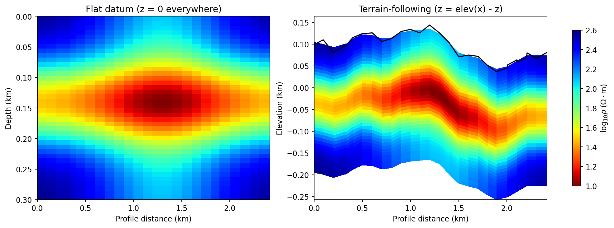
The same synthetic conductive body plotted on a flat datum (left) and in terrain-following coordinates over the real L18PLT elevation profile (right, black line). On the left it reads as a single symmetric anomaly at constant depth. On the right, the anomaly rides up and down with the terrain, most visibly where the surface drops toward the profile’s right-hand end – its depth below each station is unchanged, but its real elevation is not. Every column keeps the same 0.3 km extent, so a column under the highest terrain reaches less far down the page than one under the lowest terrain; the white wedges at bottom-left and bottom-right are simply where no cell exists at that screen position once the columns are shifted by different amounts, not a mask applied on top of the data.#
5.1.3. The PYCSAMT_TOPO singleton#
Draping is opt-in and centrally controlled. TopoConfig
follows the same configure/reset/context pattern used across
pycsamt.api: one global instance,
PYCSAMT_TOPO, decides whether topography
rendering is active for every section plot in the process, where the
elevation comes from (source="sites", "file", or "array"),
and how the terrain fill, surface line, and station pins are styled.
>>> from pycsamt.topo import PYCSAMT_TOPO, configure_topo, reset_topo

>>> PYCSAMT_TOPO.summary()
"TopoConfig(enabled=False, source='disabled', exag=1.0)"

>>> configure_topo(enabled=True, exaggeration=2.0)
>>> PYCSAMT_TOPO.summary()
"TopoConfig(enabled=True, source='sites', exag=2.0)"

>>> with PYCSAMT_TOPO.context(exaggeration=5.0):
...     print(PYCSAMT_TOPO.exaggeration)
5.0
>>> PYCSAMT_TOPO.exaggeration
2.0

>>> reset_topo()
>>> PYCSAMT_TOPO.summary()
"TopoConfig(enabled=False, source='disabled', exag=1.0)"
configure_topo() mutates the shared singleton for the rest of the
session, which is convenient in a notebook but easy to leave dirty
between figures; PYCSAMT_TOPO.context(...) scopes an override to a
single with block and restores the previous values afterwards,
even if the block raises, which is what the example above relies on to
get back to exaggeration=2.0 rather than 5.0. reset_topo()
restores every field to its package default, including enabled.
Not every section has an elevation to show. A period-versus-station
pseudosection has no vertical spatial meaning at all, so
draping it would be meaningless, and is_active_for()
exists to keep it from happening by accident:
>>> configure_topo(enabled=True)
>>> PYCSAMT_TOPO.is_active_for("depth"), PYCSAMT_TOPO.is_active_for("elevation")
(True, True)
>>> PYCSAMT_TOPO.is_active_for("period"), PYCSAMT_TOPO.is_active_for("frequency")
(False, False)
>>> reset_topo()
SectionStyle in pycsamt.api.section
wraps the same check against a section preset’s own configured
y_type as topo_active(), so
code that renders a named section preset can ask it whether draping
applies before doing any work, rather than re-deriving the depth/period
distinction itself. Turning topography on globally with
configure_topo(enabled=True) is therefore safe to leave set: a
depth or elevation section honours it, a period or frequency
pseudosection reports topo_active() == False and is left
alone. Extracting Station Topography picks up from here and covers how sites, EDI
collections, and plain arrays are each normalized into the
chain_km/elev_m pair this page has been building by hand.