5.3. Draping Flat Grids Over Terrain

Terrain-Following Coordinates introduced the transform and showed it working end to end; this page opens up pycsamt.topo.drape itself, the module that actually performs it. Four functions do the numeric work: interp_elev() turns a handful of station elevations into a value at any profile position, drape_section() uses that to warp a flat pcolormesh node grid into terrain-following coordinates, mask_above_topo() NaN-masks cells that a draped grid places above the visible terrain, and station_surface_z() returns where a station marker should sit in that same draped frame. They are small, dependency-light functions – worth reading in full, because Terrain Overlays on Section Axes and One-Call Topography-Embedded Sections are both built directly on top of them without adding any numerical logic of their own.

5.3.1. Interpolating between stations

A resistivity section rarely has one cell column per station – an Occam2D mesh usually has more columns than stations, and a synthetic grid can use any spacing at all. interp_elev() is what lets drape_section() ask “what is the terrain elevation under this column” for a position that may fall between two stations, or outside the surveyed range entirely:

>>> from pycsamt.topo import mask_above_topo

>>> query = np.array([-1.0, 0.0, 1.2, 2.418, 5.0])
>>> interp_elev(chain_km, elev_km, query)
array([0.099    , 0.099    , 0.1435964, 0.0809467, 0.081    ])
>>> elev_km[0], elev_km[-1]
(0.099, 0.081)

The two out-of-range queries, -1.0 km and 5.0 km, do not extrapolate the terrain slope outward – they clamp to elev_km[0] and elev_km[-1] respectively. An MT line is rarely surveyed with enough runout to justify guessing what the ground does beyond the first and last station, so a query past either end returns that station’s elevation flat, rather than continuing whatever local slope the last two stations happened to define. Queries between two known stations behave differently depending on method:

>>> interp_elev(chain_km, elev_km, query, method="cubic")
array([0.099     , 0.099     , 0.14408065, 0.07966647, 0.081     ])
>>> interp_elev(chain_km, elev_km, query, method="nearest")
array([0.099, 0.099, 0.144, 0.081, 0.081])

At x=1.2 km, almost exactly on station 013U (1.198 km, 144 m – the profile’s local high point from Extracting Station Topography’s figure) and just short of the next station, 014A (1.305 km, 125 m), "linear" gives 143.6 m and "cubic" gives 144.1 m – close to each other and to 013U’s own 144 m, since the query sits almost exactly on that station rather than genuinely between the two. "nearest" snaps straight to 013U’s 144 m without blending in 014A at all. The three methods disagree more at a position genuinely between two stations; both "linear" (the default) and "cubic" are reasonable choices for a smoothly rolling survey, but "cubic" needs scipy and can overshoot past a station’s elevation on a sharply irregular line, which "linear" cannot do by construction.

5.3.2. From station positions to mesh nodes

drape_section() does not stop at querying elevation for each cell centre – it needs one more elevation value per node, because pcolormesh draws an (nz, nx) grid of cells from (nz+1, nx+1) node coordinates. A small, hand-built example makes the extra interpolation step visible instead of hiding it inside a 28-station profile:

>>> x_nodes = np.array([0.0, 1.0, 2.0, 3.0])   # 4 nodes -> 3 cells
>>> z_nodes = np.array([0.0, 0.5, 1.0])         # 3 nodes -> 2 cells
>>> data = np.array([[10.0, 20.0, 30.0],
...                   [40.0, 50.0, 60.0]])       # (nz, nx) = (2, 3)
>>> elev_at_centres = np.array([0.2, 0.5, 0.1])  # one value per cell, not per node

>>> x_out, z_draped, data_out = drape_section(x_nodes, z_nodes, data, elev_at_centres)
>>> z_draped.shape
(3, 4)
>>> z_draped[0]
array([0.2 , 0.35, 0.3 , 0.1 ])

The surface row, z_draped[0], has 4 values for 3 input elevations. Internally, drape_section builds the missing node value the same way interp_elev() would: it takes the cell centre positions [0.5, 1.5, 2.5] implied by x_nodes, and linearly interpolates elev_at_centres from those onto the node positions [0.0, 1.0, 2.0, 3.0], clamping the two outer nodes to 0.2 and 0.1. Node x=1.0 sits exactly between the first two cell centres, so it becomes their average, (0.2 + 0.5) / 2 = 0.35 – not the 0.5 that a middle station actually reported. This is why Extracting Station Topography passes cell-centre positions into interp_elev() rather than reusing raw station positions directly: a single high or low station is smoothed into its neighbouring node values rather than reappearing verbatim as a sharp step in the mesh, and a mismatch between “elevation at a station” and “elevation at a nearby mesh node” of a few tens of metres is normal, not a bug, whenever the mesh spacing does not exactly match the station spacing.

Every other row of z_draped repeats the same node elevations, offset downward by that row’s depth:

>>> z_draped[1]
array([-0.3 , -0.15, -0.2 , -0.4 ])
>>> z_draped[0] - z_draped[1]
array([0.5, 0.5, 0.5, 0.5])

z_nodes[1] is 0.5, so every column in that row sits exactly 0.5 below its own surface node – confirming the transform column by column: each column keeps its own vertical offset, but every column uses the same set of relative depths.

5.3.3. Masking cells that end up above the surface

mask_above_topo() (and drape_section’s clip_above_surface=True, which calls it) exists for a specific situation: when terrain relief varies enough along a profile that a cell drawn at a plausible depth under one station ends up, once draped, sitting above the terrain surface somewhere else on the same figure. The formula is direct – a cell at row k, column j has absolute elevation elev_at_centres[j] - z_centres[k] * exaggeration, and it is masked when that value exceeds the profile’s overall maximum elevation. For an ordinary depth grid, where every z_nodes value is zero or positive, this condition can never be met, because subtracting a non-negative depth from a station’s own elevation cannot push it above the tallest station on the line – confirmed directly, even with an exaggerated 300 m outlier dropped into an otherwise flat, low profile:

>>> flat_x_nodes = np.linspace(0.0, 5.0, 11)
>>> flat_z_nodes = np.linspace(0.0, 0.4, 21)
>>> outlier_elev = np.array([0.05, 0.05, 0.05, 0.05, 0.35,
...                           0.05, 0.05, 0.05, 0.05, 0.05])
>>> flat_data = np.zeros((20, 10))
>>> masked = mask_above_topo(flat_x_nodes, flat_z_nodes, flat_data, outlier_elev)
>>> np.isnan(masked).sum()
0

Nothing gets masked, despite one column sitting 300 m above its neighbours. The masking only fires for a mesh whose z_nodes starts below zero – that is, one deliberately built to show some vertical padding above the shallowest station, rather than the ordinary “z = 0 at the surface” convention every other example on this page uses:

>>> padded_z_nodes = np.linspace(-0.2, 0.4, 21)
>>> masked_padded = mask_above_topo(flat_x_nodes, padded_z_nodes, flat_data, outlier_elev)
>>> np.isnan(masked_padded).sum(axis=0)
array([0, 0, 0, 0, 7, 0, 0, 0, 0, 0])

With that padding, the 7 rows above z = 0 under the 0.35 km-high column now exceed the profile’s own maximum elevation and are masked, while every other column – shorter than the tallest station – stays untouched. In practice this means clip_above_surface is safe to leave on by default (drape_section() and One-Call Topography-Embedded Sections’s build_topo_section() both do): it is inert for the standard grids this package produces, and only becomes active for the unusual grids where it is actually needed.

5.3.4. Vertical exaggeration, and where it does not reach

Exaggeration is meant to make thin or subtle structure visible without distorting the terrain profile into something unrecognizable. Reading drape_section’s formula again, z_draped = elev_nodes - z_nodes * exaggeration, shows why it can do both: elev_nodes (the surface) is never multiplied by exaggeration at all, only the depth term is. Plotting the surface and the deepest row at exaggeration 1, 2, and 4 on the L18PLT terrain makes the split obvious:

>>> z_nodes_flat = np.linspace(0.0, 0.3, 21)
>>> x_centres = 0.5 * (chain_km[:-1] + chain_km[1:])
>>> elev_c = interp_elev(chain_km, elev_km, x_centres)
>>> rho_flat = np.zeros((20, len(x_centres)))

>>> _, zd1, _ = drape_section(chain_km, z_nodes_flat, rho_flat, elev_c, exaggeration=1.0)
>>> _, zd2, _ = drape_section(chain_km, z_nodes_flat, rho_flat, elev_c, exaggeration=2.0)
>>> _, zd4, _ = drape_section(chain_km, z_nodes_flat, rho_flat, elev_c, exaggeration=4.0)
>>> np.allclose(zd1[0], zd2[0]), np.allclose(zd1[0], zd4[0])
(True, True)
>>> (zd1[0] - zd1[-1]).mean(), (zd2[0] - zd2[-1]).mean(), (zd4[0] - zd4[-1]).mean()
(0.3, 0.6, 1.2)

>>> fig, ax = plt.subplots(figsize=(9.5, 4.0), constrained_layout=True)
>>> _ = ax.plot(chain_km, zd1[0], color="black", linewidth=1.6,
...              label="surface (all exaggerations)")
>>> _ = ax.plot(chain_km, zd1[-1], color="#1f77b4", linewidth=1.3,
...              label="bottom, exaggeration=1")
>>> _ = ax.plot(chain_km, zd2[-1], color="#2ca02c", linewidth=1.3,
...              label="bottom, exaggeration=2")
>>> _ = ax.plot(chain_km, zd4[-1], color="#d62728", linewidth=1.3,
...              label="bottom, exaggeration=4")
>>> _ = ax.set_xlabel("Profile distance (km)")
>>> _ = ax.set_ylabel("Elevation (km)")
>>> _ = ax.set_title(
...     "Vertical exaggeration stretches relief below the surface, not the surface itself",
... )
>>> _ = ax.legend(loc="lower center", fontsize=8, ncol=2)
>>> fig.savefig("drape_exaggeration.png", dpi=170, bbox_inches="tight")

The surface row is bit-for-bit identical at every exaggeration; only the distance between it and the bottom row changes, and it scales exactly linearly – 0.3 km of depth becomes 0.6 km at exaggeration 2 and 1.2 km at exaggeration 4.

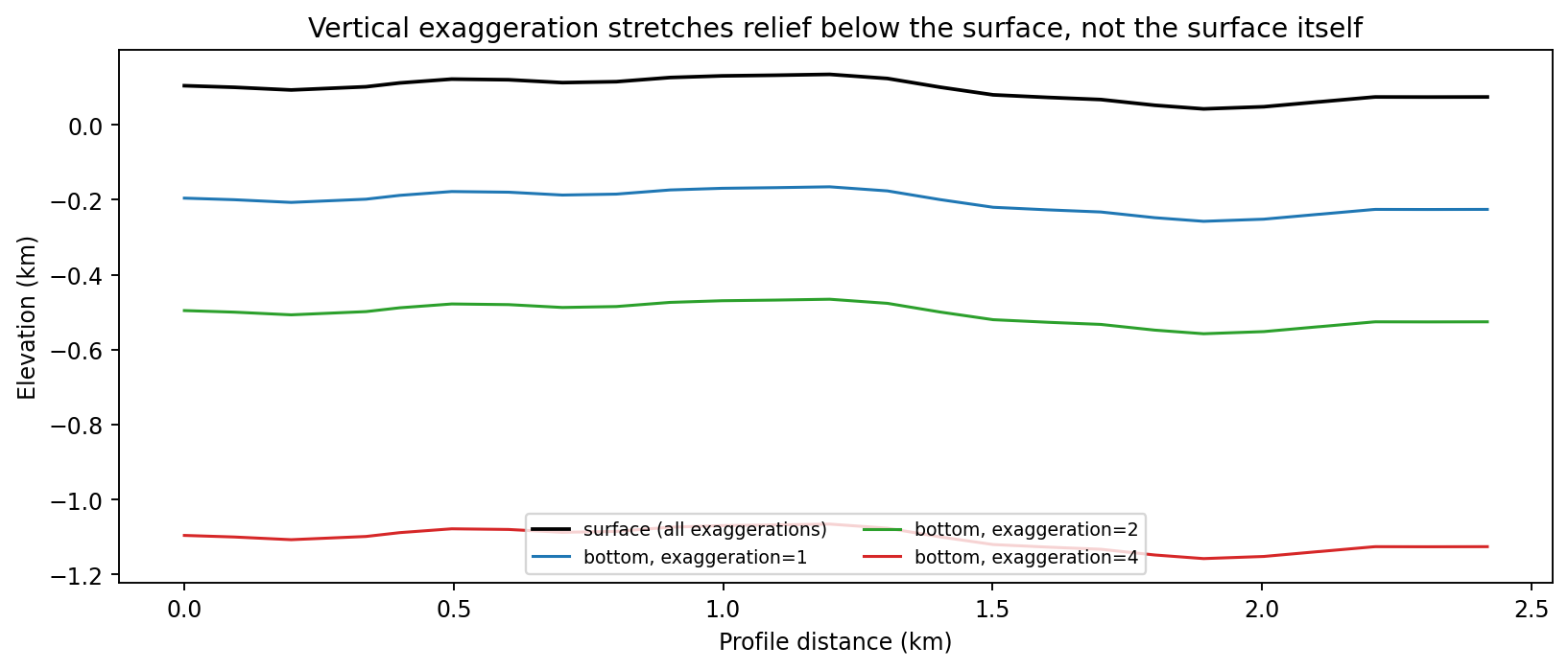
The black surface line is one curve, drawn three times, because it never moves. Each coloured line is the same flat-datum bottom row redraped at a different exaggeration – the gap it opens up below the (fixed) surface is what actually grows.

This convention belongs to drape_section alone. Both station_surface_z() and Terrain Overlays on Section Axes’s draw_topo_section() take the opposite approach, multiplying the absolute station elevation by exaggeration – elev_interp * exaggeration in the former, elev * cfg.exaggeration for the fill polygon, surface line, and station pins in the latter:

>>> from pycsamt.topo import draw_topo_section, TopoConfig

>>> tiny_chain = np.array([0.0, 1.0, 2.0])
>>> tiny_elev_m = np.array([100.0, 150.0, 120.0])

>>> fig, ax = plt.subplots()
>>> _ = ax.set_ylim(0.0, 0.3)
>>> draw_topo_section(ax, tiny_chain, tiny_elev_m, cfg=TopoConfig(exaggeration=2.0))
>>> ax.lines[0].get_ydata()
array([0.2 , 0.3 , 0.24])
>>> tiny_elev_m / 1000.0 * 2.0
array([0.2 , 0.3 , 0.24])

At exaggeration=1 this agrees with drape_section exactly, since multiplying by 1 changes nothing – the case every example before this one has used. At any other exaggeration the two genuinely disagree: a draw_topo_section terrain line drawn with cfg.exaggeration=2 would sit visibly off of a drape_section(..., exaggeration=2) mesh’s own surface row, because one scales absolute elevation and the other does not touch it at all. One-Call Topography-Embedded Sections’s plot_topo_section() avoids the mismatch by construction rather than by reconciling the two conventions: it never forwards its own exaggeration argument into the TopoConfig it builds for the draw_topo_section call, so that call always runs at the neutral exaggeration=1.0 and draws the overlay at plain, unscaled elevation – which is exactly what a drape_section surface row reduces to regardless of its own exaggeration. It is a deliberate omission, not an oversight; wiring the two exaggeration values together would reintroduce the mismatch this example demonstrates. Calling draw_topo_section or station_surface_z directly against a drape_section mesh, outside of plot_topo_section, needs the same care – pass exaggeration to at most one of the two calls, or leave both at their default of 1.0.

Terrain Overlays on Section Axes picks up here and covers draw_topo_section() and draw_topo_strip(), the two functions that turn a drape_section result (or, for the strip, a plain station index) into the filled terrain polygon, surface line, and station pins seen in every figure on this page so far.