18.12. Prepare A MARE2DEM Inversion

The two previous tutorials prepared Occam2D and ModEM runs. MARE2DEM is the third classical engine pyCSAMT integrates, and its practical entry point is different from both: rather than a mesh built automatically from station spacing, MARE2DEM starts from a resistivity grid and topology the user assembles explicitly, then triangulates through a PSLG .poly file. This tutorial builds that file set from a real single-line AMT profile, the WILLY L22PLT line – 25 stations bundled with pyCSAMT, not synthetic data.

1. load and QC one AMT profile;

2. convert it to a native MARE2DEM .emdata file with make_mt_data_from_edi(), an EDI bridge that mirrors the ZMM path already documented for MARE2DEM;

3. reason about a starting resistivity grid from the line’s own station spacing and apparent-resistivity range;

4. build the .poly/.resistivity/.settings files with grid_to_mare2dem();

5. validate the native file set and inspect the triangulation boundary;

6. hand a dry-run command to an external MARE2DEM executable.

Like Prepare an Occam2D Inversion and Prepare A ModEM Inversion, this stops short of actually running MARE2DEM – pyCSAMT does not vendor a compiled binary, and this documentation build has none either. See Run Classical Inversions: Occam2D, ModEM, and MARE2DEM for what happens once a real executable is available, and note up front that MARE2DEM is the one classical engine here without CLI support: everything below is Python only.

18.12.1. What You Will Learn

After this tutorial you should be able to:

• convert a real EDI profile into a MARE2DEM .emdata file with make_mt_data_from_edi(), and know how its station-name, TE/TM, and error-floor conventions map from the underlying EDI impedances;

• design a Y/Z resistivity grid whose cell size and padding are justified by the line’s own station spacing and skin depth range;

• turn that grid into a native MARE2DEM file set with grid_to_mare2dem(), and read back how many triangulation nodes, segments, and free/fixed regions it produced;

• recognize two real naming inconsistencies between grid_to_mare2dem’s output and Mare2DEMConfig before they cause a failed run;

• inspect the .poly boundary at both the full padded extent and the zoomed-in core region, and know why the first view alone is misleading;

• build a dry-run Mare2DEMRunner command for the file set prepared here.

18.12.2. When To Prepare A MARE2DEM Run

L22PLT is a single profile line, the same kind of geometry Prepare an Occam2D Inversion used for Occam2D. The choice between the two engines for a profile-shaped survey is rarely about the data – both read the same impedances – and mostly about what the deliverable needs to be:

• an Occam2D run gives a smooth, regularized rectangular-cell section;

• a MARE2DEM run gives an adaptive triangular-element section that can carry topography, bathymetry, and irregular boundaries explicitly, at the cost of managing an external MPI build and a genuine finite-element mesh instead of a rectangular grid.

Choosing A Model Backend frames MARE2DEM as the right choice “when the native file set and engine-specific control are part of the scientific workflow” – true here as soon as the .poly geometry itself, not only the inverted model, becomes something worth reviewing and archiving.

18.12.3. Load And QC The Profile

Loading and QC follow the same path as the Occam2D and ModEM tutorials – pycsamt.api.read_edis() followed by pycsamt.emtools.qc.station_confidence_table() – pointed at one WILLY line directory this time.

>>> from pathlib import Path

>>> from pycsamt.api import read_edis
>>> from pycsamt.emtools.qc import station_confidence_table

>>> run_root = Path("runs")
>>> run_root.mkdir(exist_ok=True)

>>> survey = read_edis(
...     "data/AMT/WILLY_DATA/L22PLT",
...     recursive=False,
...     strict=False,
...     progress=False,
... )
>>> sites = survey.collection
>>> print(len(sites))
25

>>> confidence = station_confidence_table(sites, method="composite", api=True)
>>> table = confidence.to_pandas(copy=True)
>>> print(round(table["confidence"].min(), 4), round(table["confidence"].median(), 4),
...       round(table["confidence"].max(), 4))
0.5419 0.6992 0.8087

Composite confidence spans 0.54 to 0.81 with a median of 0.70 – close to the L18PLT numbers from Prepare an Occam2D Inversion, and, like that line, nothing here forces a rejection before conversion.

18.12.4. Convert To Native MARE2DEM Data

make_mt_data_from_edi() is the EDI-to- MARE2DEM bridge: each EDI’s impedance tensor becomes a ZMMStation (TE from \(Z_{xy}\), TM from \(Z_{yx}\)), which then flows through the same profile-projection and error-floor pipeline the ZMM path already uses. It accepts the same kind of survey source as the Occam2D and ModEM builders – the in-memory sites collection from above, not only a bare path.

>>> from pycsamt.models.mare2dem.edi import make_mt_data_from_edi

>>> workdir = run_root / "line22_mare2dem"
>>> em = make_mt_data_from_edi(
...     sites,
...     workdir / "line22.emdata",
...     error_floor_te=0.05,
...     error_floor_tm=0.05,
... )
>>> print(em.n_mt_receivers, em.n_mt_frequencies, em.n_data)
25 53 5300

>>> freqs = em.mt.frequencies
>>> print(round(freqs.min(), 3), round(freqs.max(), 1))
1.008 10400.0

5300 rows is exactly 25 receivers x 53 frequencies x 4 – TE apparent resistivity, TE phase, TM apparent resistivity, and TM phase per station-frequency, with no tipper rows because this line’s EDIs carry none. The 5% error floors match the same order of magnitude used for Occam2D’s error_floor_rho and ModEM’s error_floor_z in the earlier tutorials.

Each receiver’s position in em.mt.receivers is already profile-projected – column 0 is the cross-profile offset, column 1 the along-profile distance – from an automatically detected line orientation, not raw latitude/longitude:

>>> import numpy as np

>>> receivers = em.mt.receivers
>>> x_profile, y_profile = receivers[:, 0], receivers[:, 1]
>>> print(round(y_profile.min(), 1), round(y_profile.max(), 1))
0.0 2351.3
>>> print(round(x_profile.min(), 1), round(x_profile.max(), 1))
-13.0 19.2

A plot in these profile coordinates – not equal-aspect, deliberately, so a small deviation is still visible – shows how close to a straight line the real receivers actually fall:

>>> import matplotlib.pyplot as plt

>>> figure_dir = workdir / "figures"
>>> figure_dir.mkdir(parents=True, exist_ok=True)

>>> fig, ax = plt.subplots(figsize=(9.0, 3.2))
>>> ax.plot(y_profile, x_profile, "o-", color="#2f6f8f", markersize=5)
>>> xlab = ax.set_xlabel("Distance along profile (m)")
>>> ylab = ax.set_ylabel("Cross-profile\noffset (m)")
>>> title = ax.set_title("L22PLT receiver layout in profile coordinates")
>>> ax.grid(True, alpha=0.3)
>>> fig.savefig(figure_dir / "receiver_profile.png", dpi=180, bbox_inches="tight")

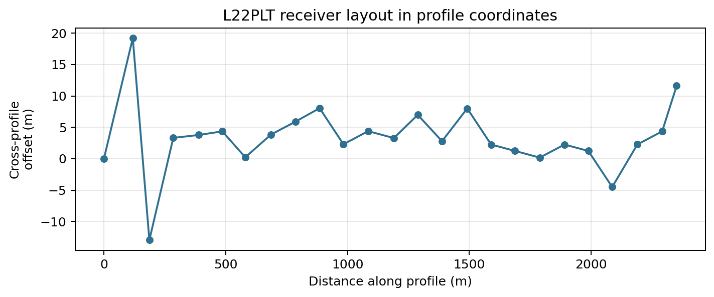
25 receivers spread over 2351 m of profile distance. Most sit within about +-10 m of the profile line, well under 1% of the line length, but one adjacent pair near 100-200 m swings from +19 m to -13 m – a real, single local kink rather than the two most distant stations, which actually sit back on-line at either end. The automatically detected line orientation is doing its job overall: this is a genuinely 2-D-appropriate profile, but that one kink is worth a field-note check before trusting a perfectly straight projection near those two stations.

18.12.5. Reason About The Starting Grid

Apparent resistivity across every TE and TM row on this line sets the same kind of skin depth argument used for the ModEM mesh in Prepare A ModEM Inversion:

>>> data = em.data
>>> rho_mask = np.isin(data[:, 0], [123, 125])
>>> rho = 10.0 ** data[rho_mask, 4]
>>> print(rho_mask.sum())
2650
>>> print(round(np.median(rho), 1), round(np.percentile(rho, 95), 1), round(rho.max(), 1))
495.5 11571.4 113086.5

Type codes 123/125 are MARE2DEM’s TE/TM log10-apparent-resistivity rows, so 10 ** data[rho_mask, 4] recovers linear \(\Omega\cdot`m directly from the data block written above. The median, 495.5 :math:\)Omegacdotmathrm{m}`, is a reasonable homogeneous starting value. The maximum, over 113000 \(\Omega\cdot\mathrm{m}\), is not: it is a handful of noisy short-period rows at the resistive tail, not evidence of a real 113 k\(\Omega\cdot\mathrm{m}\) structure, so the 95th percentile is the more defensible number for sizing how far the mesh needs to reach rather than the true maximum.

>>> from pycsamt.models.modem import skin_depth

>>> rho_median = float(np.median(rho))
>>> print(round(skin_depth(period=1.0 / freqs.max(), rho=rho_median), 1))
109.9
>>> print(round(skin_depth(period=1.0 / freqs.min(), rho=rho_median), 1))
11158.8
>>> print(round(skin_depth(period=1.0 / freqs.min(), rho=np.percentile(rho, 95)), 1))
53924.0

The shortest-period skin depth at the median resistivity is about 110 m, and the longest-period skin depth at the 95th-percentile resistivity is about 54 km. Those two numbers bound the vertical grid from both ends: cells near the top need to be a small fraction of 110 m, and whatever sits beyond the “core” grid needs to extend comfortably past 54 km before the model boundary can be treated as electromagnetically transparent – exactly the job grid_to_mare2dem’s padding region does below.

>>> y_c = np.arange(y_profile.min() - 200.0, y_profile.max() + 200.0 + 100.0, 100.0)
>>> print(len(y_c), y_c.min(), y_c.max())
29 -200.0 2600.0

>>> z_top, growth, n_z = 10.0, 1.25, 22
>>> z_c = [z_top / 2.0]
>>> thickness = z_top
>>> for _ in range(n_z - 1):
...     z_c.append(z_c[-1] + thickness / 2.0 + thickness * growth / 2.0)
...     thickness *= growth
>>> z_c = np.array(z_c)
>>> print(len(z_c), round(z_c.min(), 1), round(z_c.max(), 1))
22 5.0 4838.9

29 horizontal cells at 100 m – close to the average 98 m station spacing – cover the line plus a 200 m margin on each side. 22 vertical cells growing by a factor of 1.25 from a 5 m first cell centre reach a cell-centre depth of about 4.8 km: well past the 110 m shallow skin depth many times over, and a deliberately shallower “core” than the 54 km long-period skin depth – consistent with normal 2.5-D practice, where the core grid resolves the target depth range and a much larger fixed-resistivity padding region (added next) absorbs the far-field boundary condition instead.

18.12.6. Build The Mesh And Starting Model

grid_to_mare2dem() turns the Y/Z/Rho grid into the triangulation boundary (.poly), a homogeneous starting model (.resistivity), and a .settings file in one call.

>>> from pycsamt.models.mare2dem.grid_to_m2d import grid_to_mare2dem

>>> Y, Z = np.meshgrid(y_c, z_c)
>>> Rho = np.full(Y.shape, rho_median)

>>> files = grid_to_mare2dem(
...     Y, Z, Rho,
...     padding_y=50000.0,
...     padding_z=50000.0,
...     out_dir=workdir,
...     model_name="line22",
...     data_file="line22.emdata",
...     target_misfit=1.0,
...     max_iterations=100,
... )
>>> for role, path in sorted(files.items()):
...     print(role, path.name)
poly line22.poly
resistivity line22.0.resistivity
settings mare2dem.settings

Two of those three names deserve a second look before they surprise anyone. resistivity came back as line22.0.resistivity, not line22.resistivity – grid_to_mare2dem always numbers its output as iteration 0, the same convention the bundled demo.0.resistivity/demo.6.resistivity samples in MARE2DEM use for iteration snapshots. And settings came back as the literal mare2dem.settings regardless of model_name="line22" – the function hard-codes that filename rather than deriving it from the model stem.

50 km of padding in both directions is comfortably past the 54 km long-period skin depth estimated above – inspect the file contents to see exactly what that padding produced:

>>> from pycsamt.models.mare2dem.iotools.poly import read_poly
>>> from pycsamt.models.mare2dem.iotools.resistivity import read_resistivity

>>> poly = read_poly(files["poly"])
>>> print(len(poly.nodes), len(poly.segments), len(poly.regions))
696 1335 640

>>> resistivity = read_resistivity(files["resistivity"])
>>> free = np.asarray(resistivity.free_parameter).ravel()
>>> print(int((free != 0).sum()), int((free == 0).sum()))
638 2

638 of the 640 regions are free parameters – the 22 x 29 grid cells built above – and exactly 2 are fixed: the air layer and the outer ground-padding region grid_to_mare2dem adds automatically, both held at a reference resistivity rather than inverted.

18.12.7. Inspect The Triangulation Boundary

plot_poly draws the PSLG geometry directly, exactly as MARE2DEM uses it. Plotting the full extent first, then zooming to the core, shows why the first view alone is misleading:

>>> from pycsamt.models.mare2dem import plot_poly

>>> fig, axes = plt.subplots(1, 2, figsize=(11.5, 5.0), constrained_layout=True)

>>> plot_poly(files["poly"], ax=axes[0])
>>> title_full = axes[0].set_title("Full padded extent")

>>> plot_poly(files["poly"], ax=axes[1])
>>> axes[1].set_xlim(-500, 2900)
>>> axes[1].set_ylim(5200, -100)
>>> title_zoom = axes[1].set_title("Zoomed to the core grid")

>>> fig.savefig(figure_dir / "poly_mesh.png", dpi=180, bbox_inches="tight")

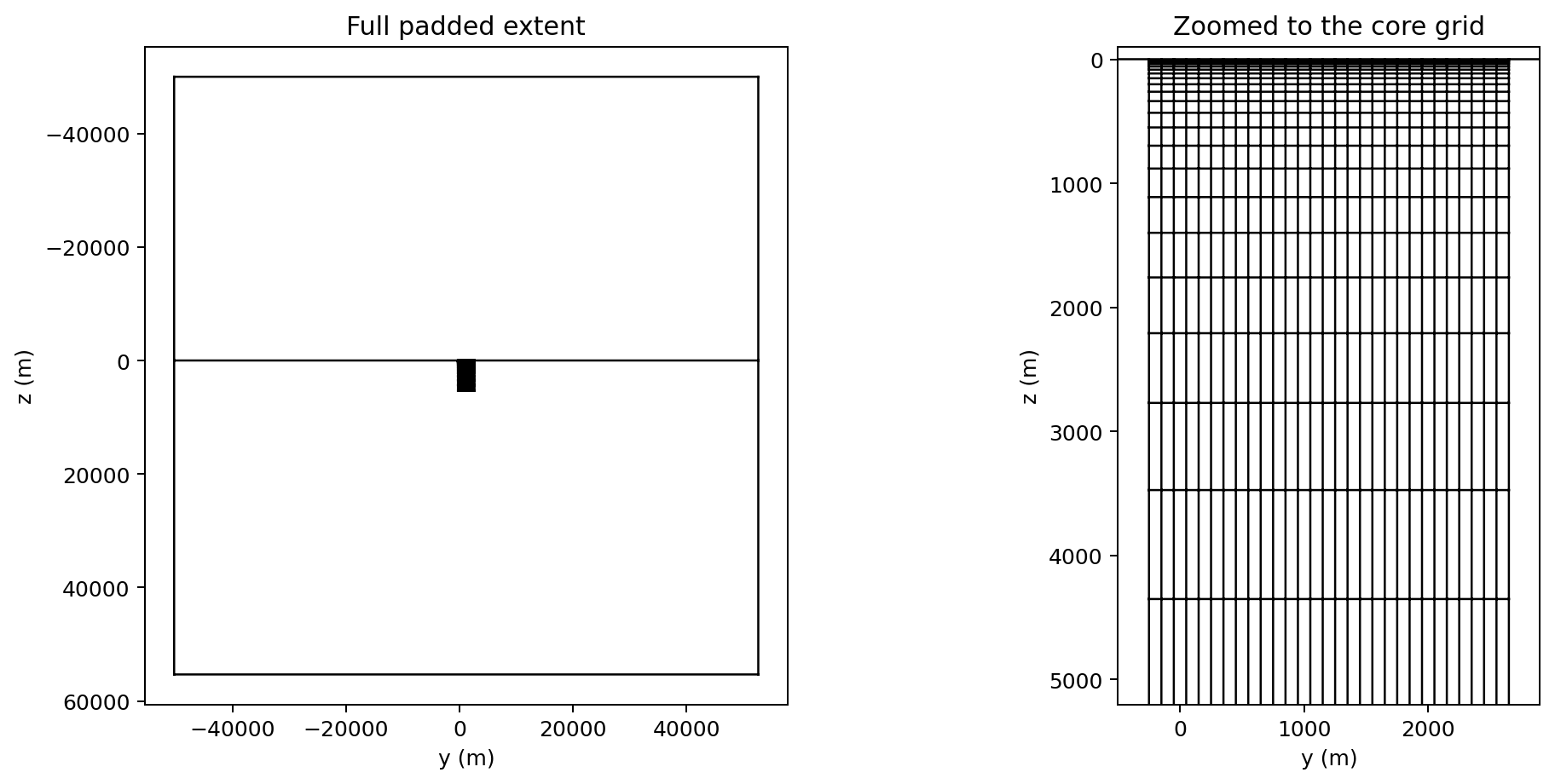
Left: the full 100 km x 100 km padded extent – the entire 2.35 km x 4.8 km core survives only as a small dark mark near the middle. That is not a plotting mistake; it is the direct, visible consequence of needing 50 km of padding on a 2.35 km line. Right: the same file, zoomed to the core region, showing the real 29-column, 22-row grid with cells thickening geometrically downward, exactly as built above. Always generate both views – the full extent to confirm the padding reaches far enough, and the zoomed view to confirm the core survived the trip intact.

18.12.8. Validate The Native Files

detect_file_type classifies MARE2DEM files by filename pattern, whether or not they exist – useful here because line22.0.resistivity and mare2dem.settings are exactly the kind of non-obvious names worth double-checking.

>>> from pycsamt.models.mare2dem import detect_file_type

>>> emdata_path = workdir / "line22.emdata"
>>> for path in (emdata_path, files["poly"], files["resistivity"], files["settings"]):
...     print(path.name, "->", detect_file_type(path))
line22.emdata -> Mare2DEMFileType.EMDATA
line22.poly -> Mare2DEMFileType.POLY
line22.0.resistivity -> Mare2DEMFileType.RESISTIVITY
mare2dem.settings -> Mare2DEMFileType.SETTINGS

All four files are recognized under their real, slightly inconsistent names – naming quirks are not the same problem as naming failures.

18.12.9. Hand Off To MARE2DEM

Mare2DEMRunner builds the exact command an external MARE2DEM executable would need. Pass the model stem directly here – "line22" – rather than Mare2DEMConfig.resistivity_stem, which would incorrectly return "line22.0" if resistivity_file were set to the .0.resistivity name grid_to_mare2dem actually wrote.

>>> from pycsamt.models.mare2dem import Mare2DEMConfig, Mare2DEMRunner

>>> cfg = Mare2DEMConfig(
...     binary="MARE2DEM",
...     use_mpi=True,
...     n_procs=8,
...     mpi_command="mpirun",
... )
>>> runner = Mare2DEMRunner(workdir, config=cfg)
>>> print(runner.command("line22"))
mpirun -np 8 MARE2DEM line22

There is no bundled MARE2DEM binary, so this is exactly what would run once a compiled executable resolves through PATH, <source_dir>/<binary>, or the platform user-data location – see MARE2DEM for SourceManager, which can download and build MARE2DEM given MPI Fortran/C tooling and Intel MKL, and Run Classical Inversions: Occam2D, ModEM, and MARE2DEM for the shared run/load recipe across all three classical engines.

18.12.10. No CLI Support Yet

Unlike Occam2D and ModEM, MARE2DEM has no pycsamt invert command-group support – --solver only accepts occam2d or modem. Everything in this tutorial is Python-only for now; there is no CLI equivalent to fall back on.

18.12.11. Preparation Checklist

Before handing this directory to a real MARE2DEM executable, confirm that:

• the line’s automatically detected orientation and profile projection look right – plot cross-profile offset, not just trust it;

• initial_rho came from the line’s own median apparent resistivity, not an arbitrary round number;

• the padded extent clears the longest-period skin depth estimated from a defensible high percentile of observed resistivity, not the raw maximum;

• the core grid’s first cell is a small fraction of the shortest-period skin depth;

• free_parameter correctly separates the real earth cells from the fixed air/padding regions;

• the resistivity file’s actual name (<model_name>.0.resistivity) and the settings file’s actual name (always mare2dem.settings) are used consistently, not assumed from Mare2DEMConfig field names;

• the runner is given the real model stem explicitly, not cfg.resistivity_stem, whenever the resistivity filename contains an iteration number;

• detect_file_type recognizes every file the run needs.

18.12.12. Troubleshooting

The resistivity filename has an unexpected .0. in it

Expected. grid_to_mare2dem always writes <model_name>.0.resistivity. Pass the plain model stem to runner.command/runner.run rather than relying on cfg.resistivity_stem.

The settings filename ignored model_name

Expected. grid_to_mare2dem always writes mare2dem.settings. Rename it after the call if a project convention needs a different name.

The full-extent .poly plot shows almost nothing

Expected once padding is many times larger than the survey. Zoom to the core region – ax.set_xlim/set_ylim after calling plot_poly – to inspect the actual grid.

The runner reports the MARE2DEM binary was not found

Expected without a locally built executable. See MARE2DEM’s SourceManager section for download/build prerequisites (MPI Fortran/C tooling, Intel MKL).

pycsamt invert build --solver mare2dem does not exist

Correct – use the Python API shown here; the CLI only wraps Occam2D and ModEM so far.

18.12.13. See Also

Prepare an Occam2D Inversion

The 2-D Occam2D counterpart to this tutorial, on a different WILLY line.

Prepare A ModEM Inversion

The 3-D ModEM counterpart, on the full five-line WILLY area survey.

Run Classical Inversions: Occam2D, ModEM, and MARE2DEM

Locating or building the MARE2DEM executable and running the files prepared here.

MARE2DEM

Full MARE2DEM backend documentation, including CSEM data, merge/noise utilities, plotting, and result loading.

Choosing A Model Backend

Deciding between Occam2D, ModEM, MARE2DEM, and other backends.

Inversion Concepts

Misfit, regularization, and inversion diagnostics referenced throughout this tutorial.

pycsamt.models

Generated API reference for the MARE2DEM objects used here.