18.11. Prepare A ModEM Inversion

The previous tutorial built a 2-D Occam2D run from a single AMT profile. Many surveys are not single profiles, though: stations are laid out over an area to resolve structure that also varies across strike, and a smooth 2-D section along one line cannot represent that. This tutorial prepares a 3-D ModEM run for exactly that case, using the real five-line WILLY AMT survey bundled with pyCSAMT. It follows the same practical arc as the Occam2D tutorial, but the center of gravity is different: building a defensible 3-D mesh is most of the work, and the native ModEM file set follows once the mesh and data selection are settled.

1. load and QC the full multi-line AMT survey;

2. choose a ModEmConfig for a 3-D run, reasoning from the data’s own frequency band and resistivity range rather than from defaults;

3. build the native data, model, covariance, and control files with InputBuilder;

4. inspect the resulting horizontal and vertical grids before trusting them;

5. validate the native file set and hand a dry-run command to an external ModEM executable;

6. reproduce the same build from the CLI.

ModEM is an external inversion program, like Occam2D. pyCSAMT prepares, validates, and can launch a run, but it does not ship a compiled Mod3DMT or Mod2DMT binary – see Run Classical Inversions: Occam2D, ModEM, and MARE2DEM once the files built here are ready to hand off.

18.11.1. What You Will Learn

After this tutorial you should be able to:

• decide when an area survey calls for a 3-D ModEM run rather than a 2-D profile inversion;

• build a ModEmConfig whose horizontal cell size, padding, air layers, and depth growth are justified by the survey’s own station spacing and skin depth range, not copied from an example;

• build the full native file set with InputBuilder and know which files are written for a 3-D run;

• read x_widths/y_widths/z_widths off the built model to check a mesh before it is sent anywhere near a solver;

• recognize which configuration fields actually control the 3-D horizontal grid and which ones do not, so tuning effort goes to the right knob;

• validate native ModEM files with detect_file_type and reproduce the same build from pycsamt invert build.

18.11.2. When A 3-D ModEM Run Is The Right Preparation

The WILLY dataset used here is not one profile: it is five parallel lines (18, 22, 26, 30, 34), 128 stations in total, spread over an area rather than strung along a single azimuth. That geometry is the practical trigger for choosing ModEM over Occam2D – Choosing A Model Backend frames the same decision as “area survey or strong 3-D structure means ModEM; profile-scale MT/AMT/CSAMT means Occam2D.” A 2-D inversion of any single WILLY line would have to ignore what the other four lines say about structure away from strike; a 3-D ModEM run uses all five at once.

18.11.3. Load The Area Survey

Loading and QC follow the same path as every earlier tutorial – pycsamt.api.read_edis() followed by pycsamt.emtools.qc.station_confidence_table() – pointed at the parent WILLY_DATA folder instead of one line subfolder, with recursive=True so all five line directories are pulled in together.

>>> from pathlib import Path

>>> from pycsamt.api import read_edis
>>> from pycsamt.emtools.qc import station_confidence_table

>>> run_root = Path("runs")
>>> run_root.mkdir(exist_ok=True)

>>> survey = read_edis(
...     "data/AMT/WILLY_DATA",
...     recursive=True,
...     strict=False,
...     progress=False,
... )
>>> sites = survey.collection
>>> print(len(sites))
128

>>> confidence = station_confidence_table(sites, method="composite", api=True)
>>> table = confidence.to_pandas(copy=True)
>>> print(table[["station", "confidence", "coverage"]].head(5).to_string(index=False))
station  confidence  coverage
18-001A    0.709038       1.0
18-002U    0.774634       1.0
18-003A    0.713303       1.0
18-004A    0.732182       1.0
18-005U    0.771060       1.0

>>> print(round(table["confidence"].min(), 4), round(table["confidence"].median(), 4),
...       round(table["confidence"].max(), 4))
0.5042 0.6795 0.8119

Composite confidence spans 0.50 to 0.81 across the survey with a median of 0.68 – lower and more scattered than the single-line L18PLT numbers in Prepare an Occam2D Inversion, which is expected once four more lines with their own noise conditions are folded in. Nothing here crosses a rejection threshold, so the full 128-station set moves forward unfiltered; a real project would still want to look at the low-confidence tail station by station before committing to a production mesh.

18.11.4. Choose A ModEM 3-D Configuration

ModEmConfig is the same source-of-truth object documented in ModEM. What changes between projects is not which fields exist, but what values are defensible for this survey – and that means looking at the data before picking numbers.

The station footprint, read directly off the built data object further down, is about 2715 m north-south by 852 m east-west: a long, narrow area, not a square grid. The retained AMT band spans the EDIs’ own native range, 1.0 Hz to 10400 Hz, and apparent resistivity across all 128 stations ranges from about 25 to 3700 \(\Omega\cdot\mathrm{m}\), with a median near 250 \(\Omega\cdot\mathrm{m}\). That median is a reasonable half-space starting value: an inversion has to move away from \(\rho_0\) in either direction, and starting near the middle of the observed range asks less of the early iterations than starting at either extreme.

The skin depth relation \(\delta \approx 503\sqrt{\rho/f}\) turns that resistivity range and frequency band into concrete depth requirements. At the shortest period (10400 Hz) and the median resistivity, \(\delta \approx 78\,\mathrm{m}\) – so a 10 m first earth layer resolves the shallowest structure several times over. At the longest period (1 Hz), \(\delta \approx 7958\,\mathrm{m}\) at 250 \(\Omega\cdot\mathrm{m}\), growing to roughly 30.6 km at the most resistive stations. The mesh built below has to reach comfortably past that number, not just past the median case.

>>> from pycsamt.models.modem import ModEmConfig

>>> cfg = ModEmConfig(
...     mode="3d",
...     component_type="Full_Impedance",
...     error_floor_z=0.05,
...     freq_min=1.0,
...     freq_max=10400.0,
...     initial_rho=250.0,
...     n_airlayers=6,
...     cell_size_h=100.0,
...     cell_size_v_top=10.0,
...     depth_scale=1.2,
...     n_padding_xy=7,
...     nz=30,
...     smooth_x=0.3,
...     smooth_y=0.3,
...     smooth_z=0.3,
...     n_smooth_iter=2,
...     max_iterations=100,
...     target_rms=1.05,
...     binary_3d="Mod3DMT",
...     use_mpi=True,
...     n_procs=16,
... )
>>> workdir = run_root / "willy_modem_3d"
>>> cfg.write_template(workdir / "modem_config.yml")

component_type="Full_Impedance" keeps all four impedance components rather than only the off-diagonal pair – appropriate here because a five-line area deployment cannot lean on a single presumed strike direction the way a rotated 2-D profile can. error_floor_z=0.05 is a 5% relative error floor, the same order of magnitude used for the Occam2D error_floor_rho in the previous tutorial. nz=30 earth layers growing by depth_scale=1.2 from a 10 m top cell is the vertical side of the skin depth argument above; the horizontal side – cell_size_h and n_padding_xy – is worth checking against the built model rather than taken on faith, which is exactly what the next two sections do.

18.11.5. Build The Native Input Set

InputBuilder turns cfg and sites into the standard 3-D file set in one call: observed data, a half-space starting model, a covariance file, and an inversion-control file.

>>> from pycsamt.models.modem import InputBuilder

>>> builder = InputBuilder(config=cfg)
>>> files = builder.build(
...     sites,
...     workdir=workdir,
...     data_filename="ModEMData.dat",
...     model_filename="m0.ws",
...     cov_filename="ModEM.cov",
...     ctrl_filename="ModEM.inv",
... )
>>> for role, path in sorted(files.items()):
...     print(role, path.name)
control ModEM.inv
covariance ModEM.cov
data ModEMData.dat
model m0.ws

>>> data, model = builder.data, builder.model
>>> print(data.n_sites, data.n_periods, data.component_types)
128 53 ['Full_Impedance']

All 53 native periods survive the freq_min/freq_max filter because the retained band matches the EDIs’ own recorded range – no data was trimmed here, only selected. builder.data, builder.model, builder.covariance, and builder.control stay attached to the builder for the inspection that follows.

18.11.6. Inspect The Horizontal Grid

ModEmModel3D.halfspace (called internally by build) derives the horizontal station-zone grid from the unique station coordinates in data.x_coords/data.y_coords, then adds n_padding_xy geometrically growing cells on each side using cell_size_h as the seed width.

>>> print(model.shape)  # (nz, ny, nx)
(36, 95, 117)
>>> print(model.n_air)
6
>>> print(round(model.x_nodes[-1]), round(model.y_nodes[-1]))
53515 51652

A plan-view map of the stations, and the same footprint with the mesh drawn on top, makes the station-zone/padding split concrete instead of abstract:

>>> import matplotlib.pyplot as plt
>>> import numpy as np

>>> figure_dir = workdir / "figures"
>>> figure_dir.mkdir(exist_ok=True)

>>> line_colors = {
...     "18": "#2f6f8f", "22": "#c85745", "26": "#3f8f61",
...     "30": "#d5962c", "34": "#7c4d79",
... }
>>> def line_code(name):
...     for part in name.split("-"):
...         if part in line_colors:
...             return part
...     return "?"

>>> names = data.site_names
>>> x, y = data.x_coords, data.y_coords  # local northing, easting (m)
>>> codes = np.array([line_code(n) for n in names])

>>> fig, axes = plt.subplots(1, 2, figsize=(11.5, 4.6), constrained_layout=True)
>>> for code, color in line_colors.items():
...     mask = codes == code
...     axes[0].scatter(
...         y[mask], x[mask], s=18, color=color,
...         edgecolor="#27323a", linewidth=0.3, label=f"Line {code}",
...     )
>>> title0 = axes[0].set_title("WILLY area survey: 5 lines, 128 stations")
>>> xlab0 = axes[0].set_xlabel("Local easting (m)")
>>> ylab0 = axes[0].set_ylabel("Local northing (m)")
>>> axes[0].set_aspect("equal", adjustable="datalim")
>>> leg0 = axes[0].legend(fontsize=8)
>>> axes[0].grid(True, alpha=0.3)

>>> x_nodes = model.x_nodes - model.x_nodes[0]
>>> y_nodes = model.y_nodes - model.y_nodes[0]
>>> x0 = x.min() - (x_nodes[-1] - (x.max() - x.min())) / 2.0
>>> y0 = y.min() - (y_nodes[-1] - (y.max() - y.min())) / 2.0
>>> x_nodes, y_nodes = x_nodes + x0, y_nodes + y0
>>> window = 400.0
>>> xlim = (x.min() - window, x.max() + window)
>>> ylim = (y.min() - window, y.max() + window)
>>> for xv in x_nodes[(x_nodes >= xlim[0]) & (x_nodes <= xlim[1])]:
...     axes[1].axhline(xv, color="#9aa4ab", linewidth=0.4)
>>> for yv in y_nodes[(y_nodes >= ylim[0]) & (y_nodes <= ylim[1])]:
...     axes[1].axvline(yv, color="#9aa4ab", linewidth=0.4)
>>> for code, color in line_colors.items():
...     mask = codes == code
...     axes[1].scatter(
...         y[mask], x[mask], s=14, color=color,
...         edgecolor="#27323a", linewidth=0.3,
...     )
>>> axes[1].set_xlim(*ylim)
>>> axes[1].set_ylim(*xlim)
>>> axes[1].set_aspect("equal", adjustable="box")
>>> title1 = axes[1].set_title("Horizontal mesh near the station footprint")
>>> xlab1 = axes[1].set_xlabel("Local easting (m)")
>>> ylab1 = axes[1].set_ylabel("Local northing (m)")

>>> fig.savefig(figure_dir / "station_footprint.png", dpi=180, bbox_inches="tight")

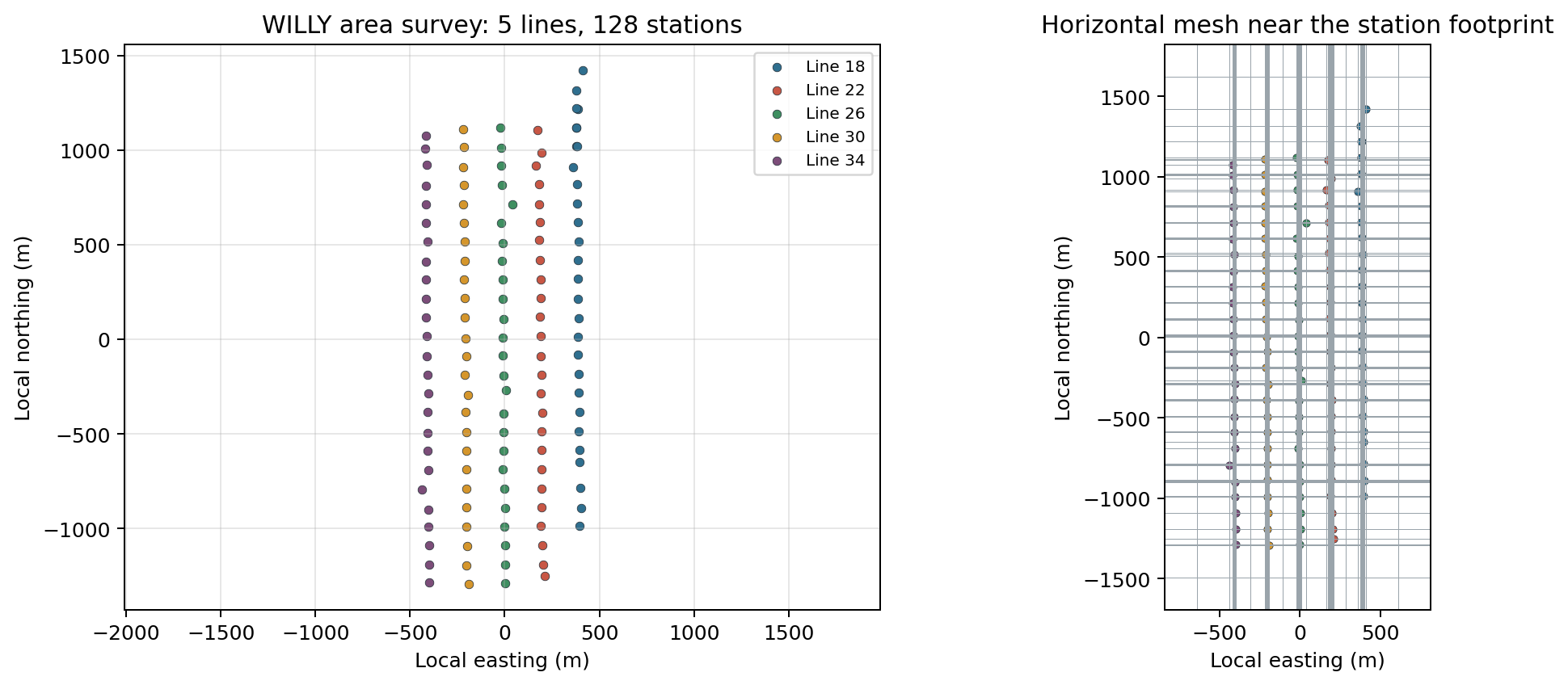
Left: all 128 stations across the five WILLY lines, in local north/east metres – a footprint about 2.7 km long and well under 1 km wide. Right: the same stations with the horizontal mesh overlaid, zoomed to the station zone plus the first padding rings (the mesh keeps growing well past this window on every side). Most cells sit close to the nominal 100 m width, but a handful come out much thinner where two stations from different lines happen to land at very similar northing or easting – worth a glance before a production run, since a very thin cell next to a 100 m one is a sharp jump in the numerical grid.

The two mesh dimensions in model.shape – ny=95 and nx=117 – are worth checking against cfg.nx and cfg.ny, because they will not match:

>>> from pycsamt.models.modem import ModEmData, ModEmModel3D

>>> for nx_probe, ny_probe in ((5, 5), (500, 500)):
...     probe_cfg = ModEmConfig(
...         mode="3d", nx=nx_probe, ny=ny_probe,
...         cell_size_h=cfg.cell_size_h, n_padding_xy=cfg.n_padding_xy,
...         n_airlayers=cfg.n_airlayers, cell_size_v_top=cfg.cell_size_v_top,
...         depth_scale=cfg.depth_scale, nz=cfg.nz,
...         freq_min=cfg.freq_min, freq_max=cfg.freq_max,
...     )
...     probe_data = ModEmData.from_edi(sites, config=probe_cfg)
...     probe_model = ModEmModel3D.halfspace(probe_data, config=probe_cfg)
...     print(f"cfg.nx={nx_probe} cfg.ny={ny_probe} -> model.shape={probe_model.shape}")
cfg.nx=5 cfg.ny=5 -> model.shape=(36, 95, 117)
cfg.nx=500 cfg.ny=500 -> model.shape=(36, 95, 117)

The shape does not move. ModEmModel3D.halfspace never reads cfg.nx or cfg.ny when it builds the 3-D horizontal grid from station coordinates – those two fields describe a core cell count that the current 3-D builder does not apply. The two levers that do change nx/ny are cell_size_h (the nominal station-zone and padding seed width) and the station coordinates themselves; pycsamt invert build reflects exactly this split, since its ModEM options are --cell-size and --n-layers with no --nx/--ny flag at all. Size a 3-D ModEM horizontal grid by choosing cell_size_h and then reading the resulting model.shape back, rather than by setting nx/ny and expecting them to hold.

The total padded extent, 53.5 km by 51.7 km, looks disproportionate next to a 2.7 km by 0.85 km station footprint, but that is what padding cells doubling in width on each of 7 rings do to a 100 m seed – and it is not excessive here, since the 30.6 km skin depth estimated above for the most resistive stations needs padding to extend nearly that far before the model’s outer boundary can be treated as electromagnetically transparent.

18.11.7. Inspect The Vertical Grid And Skin Depth

The vertical grid is simpler to reason about because cfg.nz is the number of earth layers used directly, with no equivalent surprise:

>>> earth_depth = model.z_nodes[-1] - model.z_nodes[model.n_air]
>>> print(round(model.z_widths[model.n_air], 1), round(model.z_widths[-1], 1))
10.0 1978.1
>>> print(round(earth_depth))
11819

The layer thicknesses on their own do not say whether the grid is adequate; laying them next to the skin depth curves computed above does:

>>> from pycsamt.models.modem import skin_depth

>>> fig, axes = plt.subplots(1, 2, figsize=(11.5, 4.4), constrained_layout=True)

>>> z_nodes = model.z_nodes
>>> depth = z_nodes - z_nodes[model.n_air]  # 0 at the surface
>>> layer_index = np.arange(len(depth))
>>> axes[0].step(depth, layer_index, where="post", color="#2f6f8f", linewidth=1.4)
>>> axes[0].axhline(model.n_air - 0.5, color="#c85745", linewidth=1.0, linestyle="--")
>>> boundary_text = axes[0].text(
...     depth[-1] * 0.5, model.n_air - 0.5, " air / earth boundary",
...     color="#c85745", fontsize=8, va="bottom",
... )
>>> axes[0].set_xscale("symlog", linthresh=100)
>>> xlab2 = axes[0].set_xlabel("Depth relative to surface (m)")
>>> ylab2 = axes[0].set_ylabel("Layer index (top to bottom)")
>>> title2 = axes[0].set_title(
...     f"Vertical grid: {model.n_air} air + {model.nz - model.n_air} earth layers"
... )

>>> periods = data.periods
>>> p_grid = np.geomspace(periods.min(), periods.max(), 200)
>>> for rho, color, label in (
...     (25.0, "#d5962c", r"$\rho=25\,\Omega\cdot$m (min observed)"),
...     (250.0, "#2f6f8f", r"$\rho=250\,\Omega\cdot$m (median, used as $\rho_0$)"),
...     (3700.0, "#7c4d79", r"$\rho=3700\,\Omega\cdot$m (max observed)"),
... ):
...     deltas = [skin_depth(period=float(p), rho=rho) for p in p_grid]
...     axes[1].plot(p_grid, deltas, color=color, linewidth=1.5, label=label)
>>> axes[1].axhline(earth_depth, color="#27323a", linewidth=0.9, linestyle="--")
>>> depth_text = axes[1].text(
...     periods.max(), earth_depth * 0.72, f"mesh reaches {earth_depth / 1000.0:.1f} km ",
...     fontsize=8, color="#27323a", ha="right", va="top",
... )
>>> axes[1].set_xscale("log")
>>> axes[1].set_yscale("log")
>>> xlab3 = axes[1].set_xlabel("Period (s)")
>>> ylab3 = axes[1].set_ylabel(r"Skin depth $\delta \approx 503\sqrt{\rho/f}$ (m)")
>>> title3 = axes[1].set_title("Skin depth across the modelled period band")
>>> leg3 = axes[1].legend(fontsize=7.5, loc="lower right")

>>> fig.savefig(figure_dir / "vertical_grid.png", dpi=180, bbox_inches="tight")

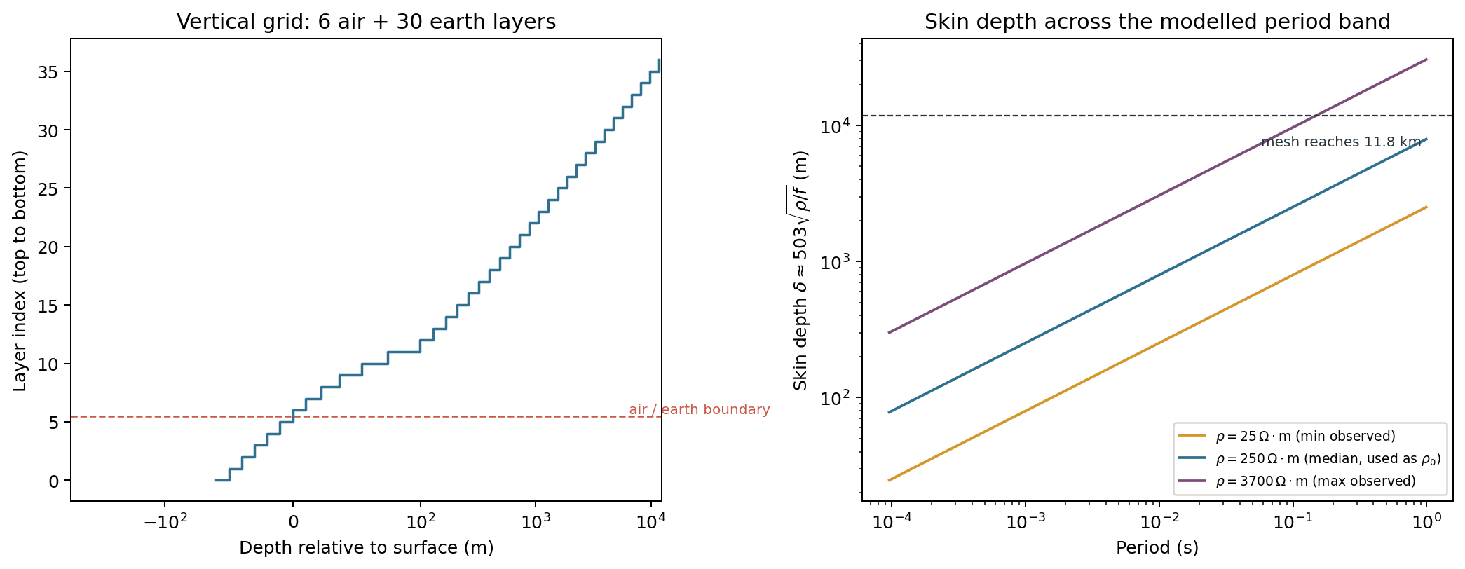
Left: the vertical grid, air layers above the dashed boundary and 30 earth layers below it, thickening geometrically from 10 m to nearly 2 km at the base. Right: skin depth versus period for the minimum, median, and maximum apparent resistivity observed across the survey, with the mesh’s 11.8 km earth-only depth marked by the dashed line. The mesh comfortably clears the skin depth curve for the median and most of the resistive stations across the whole retained period band, and only the very longest period at the single most resistive corner of the survey (the purple curve, upper right) approaches it – exactly the kind of edge case worth another look before a production run rather than a reason to distrust the mesh.

18.11.8. Covariance And Control

The 3-D build also derived a covariance file and a control file, both read straight off cfg.

>>> cov, control = builder.covariance, builder.control
>>> print(cov.nx_earth, cov.ny_earth, cov.nz_earth)
117 95 30
>>> print(cov.smooth_x[0], cov.smooth_y[0], cov.smooth_z, cov.n_smooth_iter)
0.3 0.3 0.3 2
>>> print(len(cov.mask_blocks), len(cov.exceptions))
1 0

>>> print(control.output_stem, control.initial_lambda, control.lambda_divisor)
ModEM_out 10.0 100.0
>>> print(control.target_rms, control.max_iterations)
1.05 100

cov.nz_earth equals cfg.nz exactly (30), because the covariance grid is defined directly as the model’s earth layers – unlike the horizontal count, there is no separate “core cell” field to disagree with it here. One uniform mask block covers the whole earth volume with smoothing coefficient 0.3 in every direction and no exceptions; a project that expects a known geological boundary would edit cov.mask_blocks/cov.exceptions before writing, exactly as ModEM describes.

18.11.9. Validate The Native Files

detect_file_type confirms that each file pyCSAMT wrote is recognized as the native file role it claims to be – a cheap check before a directory is copied anywhere near a cluster or a colleague.

>>> from pycsamt.models.modem import detect_file_type

>>> for role, path in sorted(files.items()):
...     print(path.name, "->", detect_file_type(path))
ModEM.inv -> control
ModEM.cov -> covariance
ModEMData.dat -> data
m0.ws -> model_3d

The recognized roles say nothing about relative size, so it is worth plotting the four file sizes directly:

>>> order = ["data", "model", "covariance", "control"]
>>> sizes_kib = [files[role].stat().st_size / 1024.0 for role in order]

>>> fig, ax = plt.subplots(figsize=(7.6, 3.8))
>>> ax.bar(
...     [files[role].name for role in order],
...     sizes_kib,
...     color=["#2f6f8f", "#7c4d79", "#d5962c", "#3f8f61"],
...     edgecolor="#27323a",
...     linewidth=0.5,
... )
>>> ax.set_yscale("log")
>>> ylab4 = ax.set_ylabel("File size (KiB, log scale)")
>>> title4 = ax.set_title("Native ModEM files written by InputBuilder")
>>> fig.savefig(figure_dir / "native_file_sizes.png", dpi=180, bbox_inches="tight")

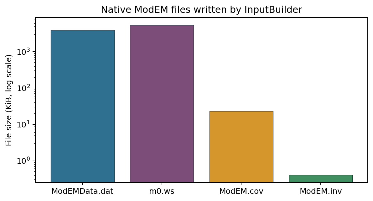
The data file (about 3.9 MiB) and starting model (about 5.4 MiB) dwarf the covariance (about 23 KiB) and control (419 bytes) files by three to four orders of magnitude – every station-period-component observation and every one of the 36 x 95 x 117 model cells is written out in full, while the covariance and control files only ever store one smoothing scheme and one set of solver settings.

18.11.10. Hand Off To ModEM

ModEmRunner builds the exact command an external Mod3DMT executable would need, without starting anything:

>>> from pycsamt.models.modem import ModEmRunner

>>> runner = ModEmRunner(workdir, config=cfg)
>>> command = runner.command("m0.ws", "ModEMData.dat", "ModEM.inv", covariance="ModEM.cov")
>>> print(command)
mpirun -np 16 Mod3DMT -I NLCG m0.ws ModEMData.dat ModEM.inv ModEM.cov

There is no bundled Mod3DMT binary, so this command is exactly what would run once a compiled executable is on PATH or in workdir – see Run Classical Inversions: Occam2D, ModEM, and MARE2DEM for locating or building it, launching it, and loading the finished run back with InversionResult.

18.11.11. CLI Equivalent

The same build reproduces from the command line, with --cell-size mapping to cell_size_h and --n-layers mapping to nz for a 3-D ModEM build:

pycsamt invert build data/AMT/WILLY_DATA \
    --solver modem --modem-mode 3d \
    --freq 1:10400 --initial-rho 250 --n-layers 30 --cell-size 100 \
    --workdir runs/willy_modem_area_cli

Inspect the working directory the same way as in the previous tutorial:

pycsamt invert status runs/willy_modem_area_cli --solver modem

invert status reports the same four files built above (data, model, covariance, control), confirms the directory is ready to run, and shows zero model files present – nothing has actually been executed yet. The CLI’s ModEM options stop at --modem-mode, --initial-rho, --freq, --n-layers, and --cell-size – there is no --n-padding, --airlayers, or --depth-scale flag. For anything beyond that minimal set, build ModEmConfig in Python (or write it to a .yml template with cfg.write_template and load it back) rather than expecting the CLI to expose every field.

18.11.12. Preparation Checklist

Before handing this directory to a real ModEM executable, confirm that:

• all lines that belong to the same 3-D deployment were loaded together (recursive=True over the whole area, not one line folder);

• component_type matches the survey’s dimensionality assumptions – full impedance for an areal deployment, off-diagonal only when a strike rotation is trusted;

• initial_rho and the retained frequency band were chosen from the data’s own resistivity and frequency range, not left at defaults;

• cell_size_h was chosen and then checked against the built model.shape, x_widths, and y_widths – not against nx/ny;

• the padded mesh extent clears the longest-period skin depth estimated from the survey’s own resistivity range;

• the vertical grid’s first layer is well below the shortest-period skin depth and the total earth depth clears the longest-period one;

• covariance smoothing values and mask regions match any known geological boundaries, or are deliberately left uniform for a first trial;

• detect_file_type recognizes every file the run needs;

• the dry-run command names the intended executable, MPI process count, and file names.

18.11.13. Troubleshooting

Changing nx/ny did not change the mesh

Expected for the 3-D builder. Change cell_size_h instead, then read model.shape back to see the effect.

The horizontal mesh has a few very thin cells

Two stations from different lines can land at very similar northing or easting after coordinate conversion. Inspect model.x_widths and model.y_widths directly and decide whether to merge nearby stations or accept the thin cells.

The padded extent looks far larger than the survey

Padding grows geometrically from cell_size_h over n_padding_xy rings specifically so the mesh boundary sits several skin depths from the stations. Compare the padded extent with skin depth at the longest retained period before assuming it is oversized.

The covariance file has only one mask block

That is the uniform default from ModEmCovariance.from_model. Edit cov.mask_blocks and cov.exceptions before writing when a known geological boundary should smooth differently.

The runner reports the ModEM binary was not found

Expected without a locally compiled Mod3DMT/Mod2DMT. See Run Classical Inversions: Occam2D, ModEM, and MARE2DEM for how the runner searches PATH, the work directory, and local _source folders.

18.11.14. See Also

Prepare an Occam2D Inversion

The 2-D Occam2D counterpart to this tutorial.

Run Classical Inversions: Occam2D, ModEM, and MARE2DEM

Locating or building the ModEM executable and running the files prepared here.

ModEM

Full ModEM backend documentation, including 2-D builds, plotting, and result loading.

Choosing A Model Backend

Deciding between Occam2D, ModEM, MARE2DEM, and other backends.

Inversion Concepts

Misfit, regularization, and inversion diagnostics referenced throughout this tutorial.

pycsamt.models

Generated API reference for the ModEM objects used here.

Inversion Commands

Inversion CLI reference.