6.3.9. Loss functions for scientific inversion

AI inversion concepts introduces a supervised objective function in two pieces, a model-space metric (6) and a response-space metric (7), and a PINN-style combination with generic vertical, lateral, and graph regularization terms (27). pycsamt.ai.losses is where that idea becomes five focused submodules with independently testable functions, reusable callable configurations, and immutable result records rather than one opaque training step:

(1)\[L = w_m L_{\mathrm{model}} + \lambda_x L_{\mathrm{grad}_x} + \lambda_z L_{\mathrm{grad}_z} + \lambda_{tv} L_{TV} + \lambda_d L_{\mathrm{response}},\]

with \(L_{\mathrm{model}}\) from model, the gradient and total-variation terms from spatial, and \(L_{\mathrm{response}}\) from response. Two further terms sit outside (1) rather than being folded into it: boundary anchors cells the training data has no sensitivity to, and uncertainty scores a network’s declared confidence, which is not something a single scalar data-fit term can express. Scalar loss functions return an immutable result record containing value, kind, reduction, n_valid, and weight_sum; depth_weights() returns an array and SpatialLoss returns its combined float directly. The counts distinguish a small fitted loss from a term that had no usable cells after masking. All five submodules operate on plain NumPy arrays; nothing here imports PyTorch or TensorFlow.

The public API is organized by the scientific question each term asks:

Family	Public interface	Question answered
Model	model_l1_loss, model_l2_loss, model_huber_loss, depth_weights, ModelLoss	How far is the predicted earth parameter grid from known training truth, after masks and scientific weights?
Spatial	gradient_smoothness_loss, total_variation_loss, SpatialLoss	How much neighboring structure or pixel-scale variation does the model contain along declared grid axes?
Boundary	boundary_condition_loss, BoundaryLoss	Does the model satisfy an explicit value on air, padding, or another constrained region?
Response	response_residual_loss, response_loss_from_contracts, ResponseLoss	Does a forward response reconstructed from the model agree with complex observations, optionally relative to their errors?
Uncertainty	gaussian_nll_loss, calibration_loss, UncertaintyLoss	Is a predicted mean accurate at the scale of its declared variance, and do interval claims match empirical held-out coverage?

The corresponding records are ModelLossResult, SpatialLossResult, ResponseLossResult, and UncertaintyLossResult. They are frozen dataclasses: store or serialize their fields rather than mutating a result after review. ResponseLossResult.normalized additionally records whether an error array was actually applied, while SpatialLossResult.label distinguishes an axis gradient from total variation.

These values are not automatically commensurate. Model loss may be in squared log-resistivity, response loss may be squared normalized impedance, spatial loss is a grid-difference penalty, and boundary loss depends on its target parameterization. Consequently, the coefficients in (1) define both numerical scaling and scientific preference. Report the input transformation, reduction, masks, valid counts, and every coefficient; quoting only the final scalar cannot reproduce the objective.

6.3.9.1. Weighting a residual by what it means

All masked scalar families use the same weighted reductions. If \(M\) contains cells that are finite, explicitly valid, and assigned positive weight,

(2)\[L_{\mathrm{mean}}= \frac{\sum_{i\in M}w_i\ell_i}{\sum_{i\in M}w_i}, \qquad L_{\mathrm{sum}}=\sum_{i\in M}w_i\ell_i.\]

reduction="mean" is usually comparable across batch sizes or changing valid-cell counts, whereas "sum" makes a larger survey or denser mask contribute more. If no positive weight remains, the mean is nan and the sum is zero; in either case n_valid and weight_sum reveal the empty term. A training system should reject that condition rather than replace nan with zero and claim a perfect fit. Notice that n_valid counts finite mask-selected cells even when their supplied weight is zero, while weight_sum records their actual influence.

model_l1_loss(), model_l2_loss(), and model_huber_loss() share one masked, weighted reduction over a predicted and a true grid — L1 and L2 in the usual sense, and Huber blending the two,

(3)\[\begin{split}\ell_\delta(r) = \begin{cases} \tfrac12 r^2, & |r| \le \delta \\ \delta\left(|r| - \tfrac12\delta\right), & |r| > \delta, \end{cases}\end{split}\]

quadratic near zero and linear beyond the transition point \(\delta\), so a handful of badly recovered cells cannot dominate the gradient the way a pure L2 term would:

>>> import numpy as np
>>> from pycsamt.ai.losses import model_l2_loss, model_huber_loss

>>> model_l2_loss(np.array([1.0, 3.0]), np.array([1.0, 1.0])).value
2.0
>>> small = model_huber_loss(np.array([0.5]), np.array([0.0]), delta=1.0).value
>>> large = model_huber_loss(np.array([5.0]), np.array([0.0]), delta=1.0).value
>>> round(small, 3), round(large, 3)
(0.125, 4.5)

A cell can be excluded three ways — a non-finite value in either array, an explicit valid mask, or a zero weights entry — and all three compose, since a masked-out cell should never silently survive because a weight happened to be positive. depth_weights() builds one common weight pattern directly: shallow cells outweigh deep ones, proportional to \(1/(1+\text{depth index})\) and normalized to sum to one, matching the intuition that near-surface structure is both easier to recover and more heavily sampled by the data than depth is:

>>> from pycsamt.ai.losses import ModelLoss, depth_weights
>>> depth_weights(3)
array([0.54545455, 0.27272727, 0.18181818])

>>> loss = ModelLoss.with_depth_weights(n_depth=3, dimension=2, kind="l2")
>>> loss.weights.shape
(3, 1)
>>> true = np.array([[1.0, 1.0, 1.0], [2.0, 2.2, 2.0], [3.0, 3.0, 3.5]])
>>> pred = np.array([[1.1, 0.9, 1.0], [2.3, 2.0, 2.1], [2.5, 3.4, 3.6]])
>>> loss(pred, true)
ModelLossResult(value=0.04181818181818182, kind='l2', reduction='mean', n_valid=9, weight_sum=3.0)

The depth-weighted value is well below the unweighted model_l2_loss(pred, true).value of 0.0644, because most of this section’s error sits in the poorly recovered bottom row, which ModelLoss’s depth weighting deliberately discounts. ModelLoss bundles a kind, reduction, and optional fixed weights into one reusable callable, so a training loop configures it once outside the loop rather than re-passing the same keyword arguments on every batch.

Loss names become easier to reason about when their penalties and influence functions are seen together. For residual \(r\), this implementation uses \(|r|\) for L1 and \(r^2\) for L2–there is no factor of one half in L2–so their derivatives away from the L1 cusp are \(\operatorname{sign}(r)\) and \(2r\). Huber has derivative \(r\) inside \([-\delta,\delta]\) and clips to \(\delta\operatorname{sign}(r)\) outside. The exact executable for the following four-panel comparison is exposed here.

</>View penalty-anatomy source codeClick to inspect and copy the complete code

def make_losses_penalty_anatomy() -> None:
    """Visualize robust, probabilistic, and response-space loss behavior."""
    from pycsamt.ai.losses import (
        gaussian_nll_loss,
        model_huber_loss,
        model_l1_loss,
        model_l2_loss,
        response_residual_loss,
    )

    residual = np.linspace(-4.0, 4.0, 401)
    zeros = np.zeros_like(residual)
    l1 = np.array([model_l1_loss([r], [0]).value for r in residual])
    l2 = np.array([model_l2_loss([r], [0]).value for r in residual])
    huber = np.array([
        model_huber_loss([r], [0], delta=1.0).value for r in residual
    ])

    sigma = np.logspace(-2.2, 0.7, 260)
    nll = {}
    for error in (0.1, 0.5, 1.0):
        nll[error] = np.array([
            gaussian_nll_loss([error], [0.0], [np.log(s**2)]).value
            for s in sigma
        ])

    frequency = np.logspace(-1, 3, 18)
    observed = (1.0 + 0.5j) * np.sqrt(frequency / frequency.max())
    predicted = observed + (0.035 + 0.025j)
    errors = np.linspace(0.015, 0.12, frequency.size)
    raw_cell = np.abs(predicted - observed) ** 2
    normalized_cell = np.abs((predicted - observed) / errors) ** 2
    raw = response_residual_loss(predicted, observed, kind="l2")
    normalized = response_residual_loss(
        predicted, observed, errors=errors, kind="l2"
    )

    fig, axes = plt.subplots(2, 2, figsize=(12.0, 8.2))
    axes[0, 0].plot(residual, l1, label="L1")
    axes[0, 0].plot(residual, l2, label="L2")
    axes[0, 0].plot(residual, huber, label=r"Huber $\delta=1$")
    axes[0, 0].set(
        xlabel="Residual", ylabel="Per-cell penalty",
        title="Large residuals dominate L2",
    )
    axes[0, 0].set_ylim(0, 8)
    axes[0, 0].grid(alpha=0.25)
    axes[0, 0].legend()

    axes[0, 1].plot(residual, np.sign(residual), label="L1 influence")
    axes[0, 1].plot(residual, 2 * residual, label="L2 influence")
    axes[0, 1].plot(
        residual, np.clip(residual, -1, 1), label="Huber influence"
    )
    axes[0, 1].set(
        xlabel="Residual", ylabel="Derivative with respect to residual",
        title="Influence controls optimization pressure",
    )
    axes[0, 1].set_ylim(-4.5, 4.5)
    axes[0, 1].grid(alpha=0.25)
    axes[0, 1].legend()

    for error, values in nll.items():
        axes[1, 0].plot(sigma, values, label=f"|residual|={error}")
        axes[1, 0].axvline(error, color="grey", lw=0.7, alpha=0.4)
    axes[1, 0].set_xscale("log")
    axes[1, 0].set(
        xlabel="Predicted standard deviation",
        ylabel="Gaussian NLL",
        title="NLL penalizes both over- and under-confidence",
    )
    axes[1, 0].set_ylim(-2.0, 15.0)
    axes[1, 0].grid(alpha=0.25, which="both")
    axes[1, 0].legend(fontsize=8)

    axes[1, 1].plot(frequency, raw_cell, "o-", label="raw contribution")
    axes[1, 1].plot(
        frequency, normalized_cell, "s-", label="error-normalized contribution"
    )
    axes[1, 1].set_xscale("log")
    axes[1, 1].set_yscale("log")
    axes[1, 1].set(
        xlabel="Frequency (Hz)", ylabel="Per-cell L2 contribution",
        title=f"Same residual: mean raw={raw.value:.3g}, normalized={normalized.value:.2f}",
    )
    axes[1, 1].grid(alpha=0.25, which="both")
    axes[1, 1].legend(fontsize=8)
    fig.suptitle("Loss choice changes which errors drive an inversion", fontsize=13)
    fig.tight_layout()
    _save(fig, "losses_penalty_anatomy.png")

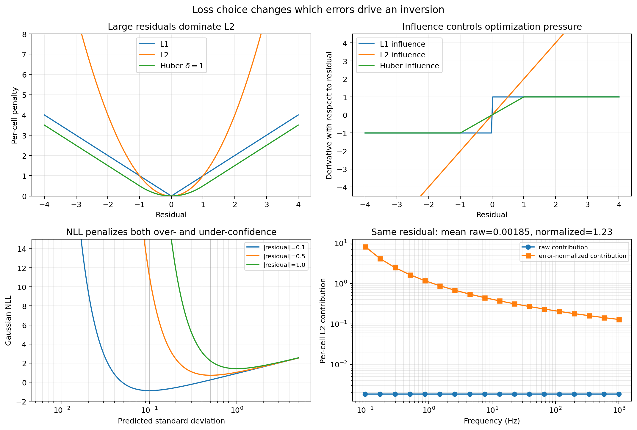
Executed loss anatomy using the public NumPy functions for every scalar value shown.

The upper panels explain why L2 rapidly redirects an optimizer toward one large residual, while L1 gives every nonzero residual equal-magnitude pressure. Huber preserves a smooth quadratic basin near the solution but limits the influence of an extreme cell. That robustness is useful for occasional target outliers, but it can also under-emphasize a real, narrow conductor if the training distribution systematically treats its large contrast as an outlier. The lower-left panel shows the uncertainty analogue: for a fixed residual the Gaussian NLL is minimized near \(\sigma=|r|\); driving variance to zero or inflating it without limit is penalized. The response panel is interpreted in detail below, where its error units are defined.

6.3.9.2. Penalizing structure, not just misfit

A network can minimize \(L_{\mathrm{model}}\) and still produce a section that is pixel-noisy between neighbouring cells that the data cannot individually distinguish. gradient_smoothness_loss() penalizes the first difference along one grid axis. For axis \(a\), it evaluates

(4)\[L_{\nabla_a}=\mathcal R\left( \ell\left[m_{\mathbf i+\mathbf e_a}-m_{\mathbf i}\right], \min(w_{\mathbf i+\mathbf e_a},w_{\mathbf i}) \right),\]

where \(\mathcal R\) is the selected reduction from (2). A pair enters only when both endpoints are finite and valid; its weight is the smaller endpoint weight. Thus a masked air cell cannot form a gradient pair with earth, and a zero-weight endpoint removes that edge. The function differences array values by cell index–it does not divide by physical dx_m, dy_m, or dz_m. On unequal cell spacing or when comparing grids, supply scientifically derived weights or implement the physical gradient explicitly.

For canonical arrays, axis 0 is depth, axis 1 is x in (z, x), and axes (0, 1, 2) are (z, y, x) in 3-D. Negative axes are accepted. The call below evaluates lateral differences along axis 1:

>>> from pycsamt.ai.losses import gradient_smoothness_loss, total_variation_loss
>>> grid = np.array([[0.0, 1.0, 3.0], [0.0, 0.0, 0.0]])
>>> gradient_smoothness_loss(grid, axis=1, kind="l1")
SpatialLossResult(value=0.75, kind='l1', label='grad_axis1', reduction='mean', n_valid=4, weight_sum=4.0)

and total_variation_loss() sums that same penalty over every axis at once — the standard anisotropic total-variation definition (a per-axis sum of directional gradients), not an isotropic pointwise gradient norm. With mean reduction it divides the sum of all directional penalties by the combined directional weight sum; it does not add separately normalized axis means. On the same predicted section used above, the three terms of (1)’s spatial part read differently depending on which direction the structure actually varies in:

>>> gradient_smoothness_loss(pred, axis=0, kind="l2").value  # depth
1.3516666666666666
>>> gradient_smoothness_loss(pred, axis=1, kind="l2").value  # lateral
0.16666666666666663
>>> total_variation_loss(pred, kind="l1").value
0.6916666666666668

The depth gradient is nearly ten times the lateral one here, because pred genuinely varies with depth by design — a reminder that \(\lambda_z\) should not, in general, be tuned to the same value as \(\lambda_x\) for a survey where vertical layering is expected and lateral continuity is the assumption worth enforcing. SpatialLoss combines all three into (1)’s \(\lambda_x L_{\mathrm{grad}_x} + \lambda_z L_{\mathrm{grad}_z} + \lambda_{tv} L_{TV}\) for a canonical 2-D (z, x) grid, and returns the combined float directly rather than a result dataclass, since it is a sum of differently-labelled terms with no single kind left to report:

>>> from pycsamt.ai.losses import SpatialLoss
>>> spatial = SpatialLoss(lambda_x=1.0, lambda_z=0.5, lambda_tv=0.1, kind="l2")
>>> spatial(pred)
0.9116666666666666

which is exactly 1.0 * 0.1667 + 0.5 * 1.3517 + 0.1 * 0.6917 from the three terms computed above — SpatialLoss is bookkeeping over the same functions, not a separate implementation. Its kind controls the x and z gradient terms, while its TV term always uses L1. It accepts only a 2-D (z, x) grid; call the lower-level axis functions directly for 3-D.

The controlled experiment below makes the trade-off concrete. A known blocky section is corrupted by cell noise and unconstrained values above a sinusoidal terrain boundary. Twenty-five Gaussian smoothing scales are treated as candidate predictions. Each candidate is scored with the public model, TV, and boundary losses, then combined with fixed coefficients. This is a diagnostic sweep, not a proposal to smooth network outputs after inference.

</>View regularization-trade-off source codeClick to inspect and copy the complete code

def make_losses_regularization_tradeoff() -> None:
    """Demonstrate data-fit versus spatial regularization on a known model."""
    from scipy.ndimage import gaussian_filter

    from pycsamt.ai.losses import (
        boundary_condition_loss,
        model_l2_loss,
        total_variation_loss,
    )

    rng = np.random.default_rng(44)
    nz, nx = 44, 76
    truth = np.full((nz, nx), 2.65)
    truth[:9] = 1.45
    truth[9:25] = 2.15
    z, x = np.mgrid[:nz, :nx]
    conductor = ((x - 38) / 15) ** 2 + ((z - 24) / 7) ** 2 <= 1
    truth[conductor] = 0.75
    noisy = truth + rng.normal(0, 0.30, truth.shape)
    air = z < (3 + 1.8 * np.sin(x / 8.0))
    noisy[air] = rng.normal(0.2, 0.35, air.sum())
    valid_earth = ~air

    scales = np.linspace(0.0, 4.0, 25)
    candidates = [noisy if scale == 0 else gaussian_filter(noisy, scale) for scale in scales]
    model_loss = np.array([
        model_l2_loss(item, truth, valid=valid_earth).value for item in candidates
    ])
    tv_loss = np.array([
        total_variation_loss(item, valid=valid_earth).value for item in candidates
    ])
    boundary_loss = np.array([
        boundary_condition_loss(item, boundary_mask=air, target=0.0).value
        for item in candidates
    ])
    lambda_tv, lambda_boundary = 0.35, 0.20
    objective = model_loss + lambda_tv * tv_loss + lambda_boundary * boundary_loss
    selected = int(np.argmin(objective))

    fig, axes = plt.subplots(2, 3, figsize=(13.2, 8.0))
    extent = [0, 7.6, 2.2, 0]
    for ax, values, title in (
        (axes[0, 0], truth, "Known blocky truth"),
        (axes[0, 1], noisy, "Noisy prediction"),
        (axes[0, 2], candidates[selected],
         f"Selected smoothing scale = {scales[selected]:.2f}"),
    ):
        image = ax.imshow(values, extent=extent, aspect="auto", cmap="turbo",
                          vmin=0.3, vmax=3.1)
        ax.contour(
            x / 10.0,
            z * (2.2 / nz),
            air,
            levels=[0.5],
            colors="white",
            linewidths=0.8,
        )
        ax.set(xlabel="Profile distance (km)", ylabel="Depth (km)", title=title)
    colorbar_axis = fig.add_axes([0.925, 0.57, 0.014, 0.29])
    fig.colorbar(image, cax=colorbar_axis,
                 label=r"$\log_{10}\rho$ [$\Omega\cdot$m]")

    axes[1, 0].plot(scales, model_loss, "o-", label=r"$L_{model}$")
    axes[1, 0].plot(scales, tv_loss, "s-", label=r"$L_{TV}$")
    axes[1, 0].plot(scales, boundary_loss, "^-", label=r"$L_{boundary}$")
    axes[1, 0].set(
        xlabel="Gaussian smoothing scale (cells)", ylabel="Mean loss",
        title="Terms prefer different models",
    )
    axes[1, 0].grid(alpha=0.25)
    axes[1, 0].legend(fontsize=8)

    axes[1, 1].plot(scales, objective, "o-", color="#7c3aed")
    axes[1, 1].axvline(scales[selected], color="#111827", ls="--")
    axes[1, 1].set(
        xlabel="Gaussian smoothing scale (cells)", ylabel="Combined objective",
        title=rf"$L_m+{lambda_tv}L_{{TV}}+{lambda_boundary}L_b$",
    )
    axes[1, 1].grid(alpha=0.25)

    scatter = axes[1, 2].scatter(
        tv_loss, model_loss, c=scales, cmap="viridis", s=55
    )
    axes[1, 2].scatter(tv_loss[selected], model_loss[selected], marker="*",
                       s=180, c="#dc2626", label="selected")
    axes[1, 2].set(
        xlabel=r"$L_{TV}$", ylabel=r"$L_{model}$",
        title="Regularity has a model-fit cost",
    )
    axes[1, 2].grid(alpha=0.25)
    axes[1, 2].legend(fontsize=8)
    fig.colorbar(scatter, ax=axes[1, 2], label="smoothing scale")
    fig.suptitle("A regularization weight selects a trade-off, not a true model", fontsize=13)
    fig.subplots_adjust(left=0.06, right=0.90, bottom=0.08, top=0.90,
                        hspace=0.34, wspace=0.31)
    _save(fig, "losses_regularization_tradeoff.png")

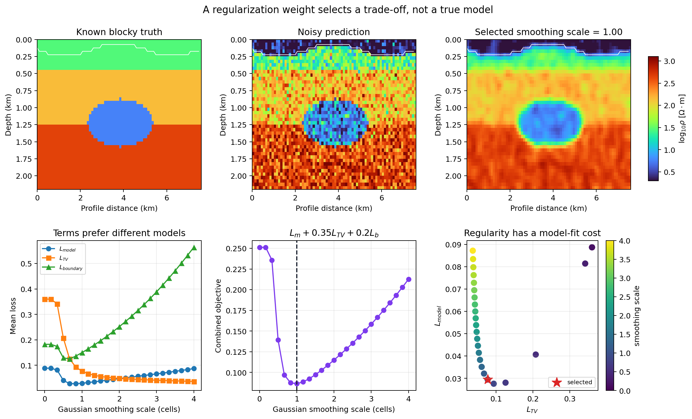
Executed regularization sweep with one common log-resistivity scale.

The unsmoothed prediction has high TV and boundary loss but is not the worst model-space fit because its sharp interfaces remain close to truth. Moderate smoothing removes pixel noise and lowers all three terms initially. Beyond the selected one-cell scale, TV continues to improve slowly while model loss rises: the conductor and layer boundaries are being blurred. The red star is selected only by \(L_m+0.35L_{TV}+0.20L_b\); changing either coefficient moves it along the trade-off curve. A low combined objective therefore identifies the preferred model under declared penalties, not the uniquely true earth.

6.3.9.3. Anchoring what the training data cannot see

Not every cell in a predicted section is constrained by the response data at all. Air cells above topography, and the outer padding of a mesh built wide enough to keep boundary effects away from the survey footprint, have no sensitivity in the forward problem — a network is free to put anything there unless something tells it otherwise. boundary_condition_loss() is a masked data-fit loss against an explicit required target value, restricted to a caller-supplied boundary_mask: there is no implicit default target, since an agent should never silently hide a physical assumption like “air is very resistive” inside a keyword default. A common source for that mask is air_mask():

>>> from pycsamt.ai.losses import BoundaryLoss
>>> air_mask = np.array([[True, True, True], [False, False, False], [False, False, False]])
>>> boundary = BoundaryLoss(kind="l1")
>>> boundary(pred, boundary_mask=air_mask, target=1.0)
ModelLossResult(value=0.0666666666666667, kind='l1', reduction='mean', n_valid=3, weight_sum=3.0)

target=1.0 here stands in for a fixed log-resistivity air value; it is chosen only to keep the arithmetic visible and is not a recommended physical air resistivity. The production target must use the same parameter space as y_pred–for example log10 resistivity if the model output is logarithmic–and must match the forward solver’s air convention. A scalar target broadcasts everywhere before the boundary mask is applied; an array target may encode a spatially varying required boundary. The small residual reflects that the top row of pred was already close to one. Internally boundary_condition_loss() reuses the exact same L1/L2/Huber machinery as model against a broadcast target array, so everything said about robust penalties and masking above applies here unchanged — a boundary constraint is a data-fit loss against a target that happens to be known in advance rather than observed.

BoundaryLoss(kind="huber", delta=...) is the reusable equivalent for repeated batches. boundary_mask itself must select at least one cell. If a separate valid mask subsequently removes every selected cell, the result follows the empty-mean behavior in (2); inspect n_valid rather than assuming the initial boundary mask guaranteed an active constraint.

6.3.9.4. Closing the loop back through the forward solver

\(L_{\mathrm{model}}\) and the spatial terms only ever look at resistivity cells; nothing yet checks whether the recovered section, run back through a solver, actually reproduces the data. response_residual_loss() closes that loop directly on complex impedance. With complex residual \(\Delta Z_i=Z_i^{\mathrm{pred}}-Z_i^{\mathrm{obs}}\), the implemented per-cell penalties are

(5)\[\ell_i^{L1}=\left|\frac{\Delta Z_i}{s_i}\right|, \qquad \ell_i^{L2}=\left(\frac{\Re\Delta Z_i}{s_i}\right)^2+ \left(\frac{\Im\Delta Z_i}{s_i}\right)^2,\]

where \(s_i=1\) without errors and otherwise is the positive absolute impedance standard error supplied for that complex cell. One scalar therefore scales both real and imaginary residuals; the function does not accept a full 2-by-2 covariance between them. L1 uses complex modulus, not separate absolute real and imaginary penalties.

>>> from pycsamt.ai.losses import response_residual_loss
>>> z_pred = np.array([1 + 1j, 2 + 2j])
>>> z_obs = np.array([1 + 1j, 0 + 0j])
>>> response_residual_loss(z_pred, z_obs, kind="l2").value
4.0
>>> response_residual_loss(z_pred, z_obs, errors=np.array([1.0, 2.0]), kind="l2").value
1.0

dividing each residual by its declared standard error before the penalty when one is supplied, matching the usual normalized-RMS EM data-misfit convention — an observation sitting at its error floor contributes less to the loss than one whose small declared uncertainty claims it should already be matched almost exactly. With kind="l2" and mean reduction, result.value is the squared normalized RMS; take sqrt(result.value) to report NRMS itself. Non-finite or non-positive error entries are excluded together with non-finite responses and valid=False cells. Always report n_valid so a lower loss cannot be mistaken for improvement when difficult observations were removed.

For repeated raw-array evaluation, configure the callable once:

>>> from pycsamt.ai.losses import ResponseLoss
>>> response_loss = ResponseLoss(kind="l2", reduction="mean")
>>> result = response_loss(
...     z_pred, z_obs, errors=np.array([1.0, 2.0]),
...     valid=np.array([True, True]),
... )
>>> result.normalized, result.n_valid, result.weight_sum
(True, 2, 2.0)
>>> np.sqrt(result.value)
1.0

response_loss_from_contracts() skips the manual array bookkeeping and takes a ForwardResult (see Solver-neutral Maxwell contracts) and a SurveyData (see Canonical data contracts) directly, refusing to run if their stations, components, or frequencies are not identically ordered — silently interpolating or reordering either axis before a misfit calculation is exactly the kind of survey-matching mistake this contract exists to rule out:

>>> from pycsamt.ai.data import SurveyData
>>> from pycsamt.forward.maxwell import ForwardResult, SolverDiagnostics
>>> from pycsamt.ai.losses import response_loss_from_contracts

>>> z = np.array([[[1 + 1j]]])
>>> observed = SurveyData(z, [10.0], ["S1"], ["zxy"], [[0, 0]])
>>> diagnostics = SolverDiagnostics([[True]], [[1]], [[0.0]], 0.01)
>>> forward = ForwardResult(
...     "a" * 64, [10.0], ["S1"], ["zxy"], z, None, "demo", "1", diagnostics,
... )
>>> response_loss_from_contracts(forward, observed).value
0.0

The lower-right panel of losses_penalty_anatomy.png holds the complex residual fixed at every frequency. Raw L2 contributions are therefore flat and their mean is 0.00185 in the example’s impedance units squared. Declared errors increase from 0.015 to 0.12, so normalization makes low-frequency cells exert far greater pressure and raises the mean normalized loss to 1.23. This is not an intrinsic frequency weighting: it is entirely induced by the supplied error array. If error floors or units are wrong, the optimizer will faithfully emphasize the wrong observations.

response_loss_from_contracts intersects forward.valid with observed.valid and uses observed.impedance_error when requested and available. Solver convergence metadata beyond that validity mask is not itself part of the scalar loss, so preserve the full SolverDiagnostics beside the result.

This is the same pairing the two-family split in Domain-gap and noise simulation exists for: a network trained only against clean synthetic responses has no reason to expect the noise, static shift, and distortion an \(L_{\mathrm{response}}\) term will encounter once observed comes from a real survey rather than another generate_2d_maxwell_dataset() sample.

6.3.9.5. Making declared uncertainty answerable to evidence

A model that predicts a resistivity value without a credible error bar is only half a result. gaussian_nll_loss() trains a heteroscedastic aleatoric uncertainty head alongside the mean prediction, with each cell contributing

(6)\[\ell_i = \tfrac12\left(\frac{(\hat y_i - y_i)^2}{\sigma_i^2} + \log\sigma_i^2 + \log 2\pi\right), \qquad \sigma_i^2 = \exp(\log\sigma_i^2),\]

parameterized through a predicted log-variance rather than the variance itself, so the network output stays unconstrained in sign while \(\sigma_i^2\) is guaranteed positive after the exponential:

>>> from pycsamt.ai.losses import gaussian_nll_loss, calibration_loss
>>> pred_u = np.array([1.0, 2.2, 2.9, 4.5])
>>> true_u = np.array([1.1, 2.0, 3.0, 4.0])
>>> log_var = np.log(np.array([0.05, 0.1, 0.2, 0.3]))
>>> gaussian_nll_loss(pred_u, true_u, log_var)
UncertaintyLossResult(value=0.09038918945783034, kind='gaussian_nll', reduction='mean', n_valid=4, weight_sum=4.0)

Unlike L1, L2, and Huber, Gaussian NLL need not be non-negative: a sufficiently accurate mean with variance below \(1/(2\pi)\) can produce a negative log density. That is not an invalid result. For one fixed nonzero residual, setting the derivative with respect to variance to zero gives \(\sigma^2=r^2\), which explains the minima in the lower-left figure. Jointly training mean and log-variance can still hide systematic mean errors behind inflated variance unless calibration and sharpness are checked on held- out data. Very large finite log-variance can also overflow exp numerically; the NumPy function does not clip it, so constrain or stabilize an autograd implementation deliberately.

UncertaintyLoss stores the reduction for repeated batches and forwards masks and weights unchanged:

>>> from pycsamt.ai.losses import UncertaintyLoss
>>> nll = UncertaintyLoss(reduction="sum")
>>> batch = nll(
...     pred_u, true_u, log_var,
...     valid=np.array([True, True, False, True]),
... )
>>> batch.reduction, batch.n_valid, round(batch.value, 6)
('sum', 3, 0.222337)

A low, well-behaved log-variance still needs checking against reality: declaring \(\sigma\) honestly is not the same as being right about it. calibration_loss() scores that separately, penalizing the gap between empirical coverage measured on a held-out calibration set and the nominal confidence level each coverage value was supposed to hit:

>>> coverage = np.array([0.42, 0.68, 0.83, 0.94])
>>> nominal = np.array([0.5, 0.7, 0.8, 0.9])
>>> calibration_loss(coverage, nominal)
UncertaintyLossResult(value=0.0023249999999999968, kind='calibration', reduction='mean', n_valid=4, weight_sum=4.0)

calibration_loss(kind="l1") uses absolute coverage error and kind="l2" uses squared error. The returned result’s kind is "calibration" in both cases, so record the selected residual kind in the experiment configuration; it cannot be reconstructed from the result record alone.

The two stay separate functions rather than one combined call deliberately: the Gaussian NLL is a per-cell term evaluated and backpropagated every training step, while calibration summarizes predictive intervals across many held-out realizations and is checked periodically, not differentiated through.

6.3.9.6. Assemble an auditable staged score

Keep component results before forming a total. This makes masks, counts, and scales inspectable and prevents a weighted sum from erasing the reason it changed:

>>> from pycsamt.ai.losses import ModelLoss, SpatialLoss, BoundaryLoss
>>> model_term = ModelLoss(kind="l2")(pred, true)
>>> spatial_term = SpatialLoss(
...     lambda_x=1.0, lambda_z=0.5, lambda_tv=0.1, kind="l2"
... )(pred)
>>> boundary_term = BoundaryLoss(kind="l1")(
...     pred, boundary_mask=air_mask, target=1.0
... )
>>> response_term = ResponseLoss(kind="l2")(
...     z_pred, z_obs, errors=np.array([1.0, 2.0])
... )
>>> terms = {
...     "model": model_term.value,
...     "spatial": spatial_term,
...     "boundary": boundary_term.value,
...     "response": response_term.value,
... }
>>> coefficients = {
...     "model": 1.0, "spatial": 0.05,
...     "boundary": 0.10, "response": 0.20,
... }
>>> total = sum(coefficients[name] * value for name, value in terms.items())
>>> {name: round(value, 4) for name, value in terms.items()}
{'model': 0.0644, 'spatial': 0.9117, 'boundary': 0.0667, 'response': 1.0}
>>> round(total, 4)
0.3167

This number is reproducible only with the arrays and conventions established earlier in the page. In production, fail the batch if any enabled component is non-finite or has zero weight_sum. Log each unweighted value, coefficient, weighted contribution, valid count, and mask identifier. Tune coefficients on validation evidence rather than choosing them merely to make printed terms similar in magnitude; equal numerical scale does not imply equal scientific importance.

6.3.9.7. Wiring the spatial terms into a trainable network

Every function above operates on NumPy arrays, which is what keeps pycsamt.ai.losses importable without an optional deep-learning backend and lets every example on this page run without one — but a NumPy array cannot participate in backpropagation. EMInverter2D’s fit method exposes lambda_x, lambda_z, and lambda_tv keywords that add the lateral-gradient, depth-gradient, and total-variation terms to its plain MSE data fit during PyTorch training, mirroring the math of (1)’s spatial part but computed directly on normalized torch tensors rather than by calling spatial itself, since a training step needs gradients to flow through the penalty and not just past it. All three weights default to zero, which reproduces plain MSE training unchanged, and the staged terms are currently only implemented for the PyTorch backend: passing a nonzero weight while TensorFlow is active raises NotImplementedError rather than silently ignoring the request. response, boundary, and uncertainty are not yet wired into that same training step; they remain available today for offline scoring — exactly the checks Recovery, residual, and OOD diagnostics runs after training, independently of whichever loss shaped it.

There are two precise differences between that training adapter and the NumPy diagnostics. The PyTorch TV adapter adds the separate mean absolute x and z gradients, whereas total_variation_loss() pools all directional differences before its mean reduction. It also operates after one global target normalization and currently accepts no validity mask or per-cell weights. Therefore the same numerical lambda_tv does not guarantee the same scalar reported by an offline call on physical log-resistivity. Use the NumPy package as the authoritative auditable diagnostic API and regard each backend training adapter as a separately versioned implementation that must be tested against its intended formula.

6.3.9.8. Choose and validate the objective deliberately

No loss family is universally best. A defensible starting decision is:

Term	Useful when	Main failure to test
Model L2	Synthetic targets are trustworthy and large errors should receive rapidly increasing pressure.	Rare contrasts or mislabeled cells dominate training.
Model L1	Robustness to sparse large target errors matters.	Constant influence slows fine convergence and underweights meaningful high-contrast bodies.
Model Huber	A smooth near-zero basin and bounded outlier influence are both useful.	delta is chosen in the wrong transformed units.
Gradient/TV	Geological continuity or piecewise-constant structure is part of the declared prior.	Thin conductors, faults, and interfaces are erased; cell spacing is ignored.
Boundary	Air, padding, or fixed regions have explicit values and masks.	A numerical target uses the wrong log/linear convention or constrains cells that should remain free.
Response	Predictions can be forwarded through verified physics on aligned survey contracts.	Incorrect errors, validity masks, solver bias, or units redirect fit.
Gaussian NLL	The network predicts both a conditional mean and heteroscedastic log-variance.	Variance inflation hides bias, or extreme log-variance overflows.
Calibration	Held-out interval coverage is available across many independent cases.	Calibration data leak into fitting or fail to represent deployment.

For synthetic training, monitor model-space recovery and response-space fit together. A model can be close cell by cell yet reproduce responses poorly if the forward operator is sensitive to a small misplaced structure; another can fit responses well while differing greatly from truth because EM inversion is non-unique. For field deployment, model loss against truth is unavailable, so response residuals, uncertainty calibration, geology, dimensionality tests, and classical baselines carry the acceptance decision. Regularization makes a solution preferable under a prior; it does not create information in the data.