Noise Removal And Spatial Filtering

pycsamt.emtools.remove_noise is the main post-estimation cleaning module for CSAMT/AMT/MT transfer functions. It operates on impedance and tipper arrays already stored in EDI or Sites objects. It does not estimate transfer functions from time series, and it does not perform true remote-reference processing internally. Use it after data loading, and before inversion or final interpretation, when the survey contains power-line harmonics, isolated frequency spikes, station-local outliers, station-to-station jumps, or rows that should be filtered more strongly because their confidence is low.

The module has many functions because noise is not one problem. A single CSAMT line may need one or more of these treatments:

Step	Use when	Typical functions
Diagnose noise	You need to see which stations and frequencies are weak before editing the survey.	snr_table, emi_mitigation_report
Remove mains harmonics	Frequencies land near 50/60 Hz or harmonics.	notch_powerline
Smooth along frequency	Curves are locally jagged, but neighboring frequencies should be continuous.	smooth_logfreq, smooth_rho_phase
Remove isolated outliers	A few rows or stations are inconsistent with their local neighbors.	hampel_filter_freq, spatial_median_filter, rpca_offdiag_denoise
Enforce impedance consistency	Off-diagonal components should be closer to an anti-symmetric 1-D/2-D response.	enforce_offdiag_consistency
Mask or drop bad frequencies	Frequencies are globally weak or known to be contaminated.	mask_incoherent_freqs, drop_freqs_manual
Stabilize station profiles	One station is shifted relative to its neighbors, or an EMAP style spatial average is appropriate.	correct_static_shift, apply_emap_filter, confidence_gated_emap_filter
Verify the correction	You need before/after figures for the report or paper.	emap_filter_report, plot_emap_filter_profile, plot_emap_filter_psection, nr_qc_* plots

Full function signatures and parameter defaults are maintained in the API reference. This page focuses on practical usage, decision making, and reproducible code.

Loading A Survey Safely

Noise removal functions accept the same inputs as most emtools workflows: a directory of EDI files, a single EDI path, an existing Sites object, or an iterable of station-like objects. For repeatable processing, load once with ensure_sites and keep the raw object unchanged while you test settings.

from pathlib import Path

from pycsamt.emtools import ensure_sites

edi_dir = Path("data/AMT/WILLY_DATA/L18PLT")
raw = ensure_sites(edi_dir, recursive=True, verbose=0)

# Most remove_noise functions default to inplace=False. The returned
# object is therefore the processed survey, while raw remains the
# baseline for before/after QC.
processed = raw

Use inplace=False during exploration. Switch to inplace=True only inside a controlled pipeline where you no longer need the raw object in memory.

SNR Diagnostics

The simplest diagnostic is snr_table. It returns one row per station and frequency. For each row, pyCSAMT computes an impedance-amplitude signal-to-noise ratio from Z and Z_err:

\[\mathrm{SNR} = \frac{\sqrt{\overline{|Z|^2}}} {\sqrt{\overline{|Z_{\mathrm{err}}|^2}}}\]

If the input EDI files do not contain impedance errors, the SNR values are NaN. That is useful information: it means later SNR-gated steps cannot make a data-driven decision from error bars.

from pycsamt.emtools import ensure_sites
from pycsamt.emtools.remove_noise import snr_table

sites = ensure_sites("data/AMT/WILLY_DATA/L18PLT", recursive=True)
snr = snr_table(sites)

print(snr.head())
print(snr["snr"].describe())

weak_rows = snr.loc[snr["snr"] < 3.0, ["station", "freq", "snr"]]
weak_by_station = (
    weak_rows.groupby("station", as_index=False)
    .agg(n_weak=("freq", "size"), min_snr=("snr", "min"))
    .sort_values(["n_weak", "min_snr"], ascending=[False, True])
)
print(weak_by_station.head(10))

station     freq        snr
0  18-001A  10400.0  24.379116
1  18-001A   8707.0  21.511108
2  18-001A   7289.0  21.241377
3  18-001A   6102.0  15.230757
4  18-001A   5108.0  13.140256
count    1484.000000
mean       14.064419
std         5.878163
min         2.187781
25%         9.679665
50%        13.271554
75%        17.294278
max        56.055512
Name: snr, dtype: float64
   station  n_weak   min_snr
2  18-024U       3  2.187781
1  18-022U       1  2.388301
0  18-018A       1  2.808353

Import snr_table from pycsamt.emtools.remove_noise when you are documenting this module specifically. The top-level pycsamt.emtools namespace also exposes an snr_table name used by the spectra tools, so the explicit module import avoids ambiguity.

Remote Reference And EMI Reporting

The remove-noise layer works on estimated transfer functions. It cannot create a remote-referenced impedance tensor unless remote-reference processing was already performed by field software or an external processor. What it can do is make the mitigation record explicit: whether remote reference was attempted, whether it was available, which power-line notch settings were used, and how many harmonic samples were affected.

from pycsamt.emtools import ensure_sites
from pycsamt.emtools.remove_noise import emi_mitigation_report

sites = ensure_sites("data/AMT/WILLY_DATA/L18PLT", recursive=True)

emi = emi_mitigation_report(
    sites,
    remote_reference_attempted=False,
    remote_reference_reason=(
        "No independent remote-reference time series were acquired; "
        "post-estimation EMI mitigation was applied to the EDI transfer functions."
    ),
    mains_hz=50.0,
    n_harm=30,
    tol_hz=0.08,
    notch_mode="interp",
)

print(
    emi[
        [
            "station",
            "remote_reference_attempted",
            "remote_reference_available",
            "n_frequency",
            "harmonic_z_samples",
            "harmonic_tipper_samples",
            "applied_measures",
        ]
    ].head()
)

   station  ...                                   applied_measures
0  18-001A  ...  notch_powerline(mode=interp, mains_hz=50, n_ha...
1  18-002U  ...  notch_powerline(mode=interp, mains_hz=50, n_ha...
2  18-003A  ...  notch_powerline(mode=interp, mains_hz=50, n_ha...
3  18-004A  ...  notch_powerline(mode=interp, mains_hz=50, n_ha...
4  18-005U  ...  notch_powerline(mode=interp, mains_hz=50, n_ha...

[5 rows x 7 columns]

This report is especially useful in manuscripts and reproducibility bundles because it states what was not done as clearly as what was done. If remote-reference EDIs are supplied, load those files and set the report fields accordingly.

Power-Line Notching

notch_powerline finds frequencies within tol_hz of mains_hz * k for harmonics k = 1 .. n_harm. It can either set those rows to NaN with mode="mask" or replace them by interpolation from neighboring frequencies with mode="interp".

from pycsamt.emtools import ensure_sites, notch_powerline

sites = ensure_sites("data/AMT/WILLY_DATA/L18PLT", recursive=True)

notched = notch_powerline(
    sites,
    mains_hz=50.0,
    n_harm=30,
    tol_hz=0.08,
    mode="interp",
    also="both",
    inplace=False,
)

Use mode="mask" when you want contaminated rows to remain visibly missing for later QC. Use mode="interp" when the downstream workflow requires a complete frequency axis. Use also="z" for impedance only, also="tipper" for tipper only, or also="both" when both tensors share the same contaminated frequencies.

Sparse logarithmic CSAMT grids often do not land exactly on 50/60 Hz harmonics. In that case the function may make no changes at conservative tol_hz values. That is not a failure. It means the sampled frequencies are not close enough to the harmonic rows you asked it to treat.

Log-Frequency Smoothing

smooth_logfreq applies a moving average directly to complex tensor rows along the frequency axis. It is a local smoother. It does not assume a global resistivity model; it only says that neighboring log-frequency samples should be less jagged.

from pycsamt.emtools import ensure_sites, smooth_logfreq

sites = ensure_sites("data/AMT/WILLY_DATA/L18PLT", recursive=True)

smoothed = smooth_logfreq(
    sites,
    win=5,
    kind="tri",
    also="both",
    gate_snr=2.5,
    inplace=False,
)

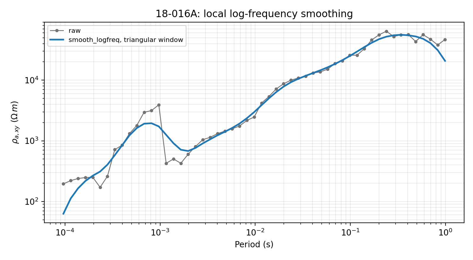
win is the number of frequency rows used by the moving window. kind="tri" gives the center row more weight than the edges; kind="box" gives every row equal weight. gate_snr limits smoothing to rows that pass the chosen SNR logic inside the function. Set gate_snr=None when you deliberately want every row smoothed.

Rho/Phase Trend Smoothing

smooth_rho_phase is more interpretive. It converts impedance components to apparent resistivity and phase, fits a polynomial trend in log-frequency space, unwraps phase, then rebuilds complex impedance from the smoothed curves.

from pycsamt.emtools import ensure_sites, smooth_rho_phase

sites = ensure_sites("data/AMT/WILLY_DATA/L18PLT", recursive=True)

trend = smooth_rho_phase(
    sites,
    components="offdiag",
    degree=3,
    min_points=None,
    smooth_rho=True,
    smooth_phase=True,
    robust=True,
    robust_iters=3,
    blend=1.0,
    inplace=False,
)

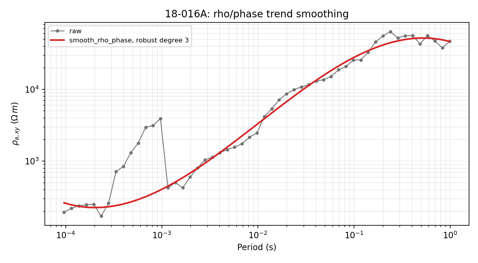
Choose smooth_logfreq for local jitter. Choose smooth_rho_phase when you expect a station curve to follow a smooth global trend. components can be "offdiag", "diagonal", "all", or an explicit list such as ("xy", "yx"). blend lets you mix the filtered value with the original value; for example blend=0.5 moves only halfway toward the fitted trend.

Outlier And Spatial Denoising

Outlier removal can operate along one station’s frequency curve, across neighboring stations, or across the whole survey matrix.

from pycsamt.emtools import (
    ensure_sites,
    hampel_filter_freq,
    rpca_offdiag_denoise,
    spatial_median_filter,
)

sites = ensure_sites("data/AMT/WILLY_DATA/L18PLT", recursive=True)

# Per-station, along frequency. Best for isolated spikes in one curve.
hampel = hampel_filter_freq(
    sites,
    win=3,
    nsig=3.0,
    on="z",
    inplace=False,
)

# Across station order. Best for a station that jumps relative to its
# neighbors at the same frequency.
spatial = spatial_median_filter(
    sites,
    half_window=2,
    lam=0.25,
    on="z",
    inplace=False,
)

# Survey-wide low-rank denoising of off-diagonal log magnitudes.
# Best when the line has a common coherent trend plus sparse outliers.
low_rank = rpca_offdiag_denoise(
    sites,
    rank=2,
    inplace=False,
)

hampel_filter_freq is conservative at typical nsig values. It does not remove a station merely because the station is high amplitude; it removes rows that are local outliers relative to the station’s own nearby frequencies. spatial_median_filter uses neighboring stations, so it should be applied only when station order has spatial meaning. rpca_offdiag_denoise can be powerful, but a low-rank model may damp a real station anomaly if that anomaly is not shared by the rest of the line. Always inspect before/after curves when using it.

Off-Diagonal Consistency

For a simple 1-D or approximately 2-D response, the off-diagonal impedance terms often satisfy an anti-symmetric relationship: Zxy ~= -Zyx. enforce_offdiag_consistency blends the observed off-diagonal components toward that target.

from pycsamt.emtools import ensure_sites, enforce_offdiag_consistency

sites = ensure_sites("data/AMT/WILLY_DATA/L18PLT", recursive=True)

consistent = enforce_offdiag_consistency(
    sites,
    mode="anti",
    lam=0.5,
    inplace=False,
)

lam=0 leaves the data unchanged. lam=1 fully replaces the selected components by the consistency target. Intermediate values are usually safer because real 3-D structure, galvanic distortion, and measurement geometry can all create departures from the ideal anti-symmetric relation.

Masking And Manual Frequency Drops

mask_incoherent_freqs uses the survey SNR table to identify frequencies where too few stations pass an SNR threshold. It masks those frequencies rather than pretending they are reliable.

from pycsamt.emtools import (
    drop_freqs_manual,
    ensure_sites,
    mask_incoherent_freqs,
)

sites = ensure_sites("data/AMT/WILLY_DATA/L18PLT", recursive=True)

masked = mask_incoherent_freqs(
    sites,
    snr_thresh=2.5,
    min_frac=0.4,
    inplace=False,
)

trimmed = drop_freqs_manual(
    sites,
    drop_freqs=[50.0, 60.0],
    tol_rel=0.005,
    inplace=False,
)

Use mask_incoherent_freqs for a rule based on the data. Use drop_freqs_manual when the field log, instrument notes, or a diagnostic figure identifies specific frequencies. Manual drops use a relative tolerance, so give the sampled frequency value when possible.

Group-Trend Shrinkage

shrink_to_group_trend pulls station curves toward a group median trend. By default it is gated to harmonic rows, which makes it a targeted EMI treatment rather than a blanket smoothing operation.

from pycsamt.emtools import ensure_sites, shrink_to_group_trend

sites = ensure_sites("data/AMT/WILLY_DATA/L18PLT", recursive=True)

harmonic_shrink = shrink_to_group_trend(
    sites,
    lam=0.25,
    gate_harm=True,
    mains_hz=50.0,
    n_harm=30,
    tol_hz=0.08,
    inplace=False,
)

all_rows_shrink = shrink_to_group_trend(
    sites,
    lam=0.25,
    gate_harm=False,
    inplace=False,
)

Keep gate_harm=True when the problem is power-line contamination. Use gate_harm=False only when you have decided that the entire line should be pulled toward a common spatial trend.

Static Shift And EMAP Filters

The module contains two related families of station-profile filters. correct_static_shift implements a Torres-Verdin and Bostick style Hanning adaptive moving-average correction. apply_emap_filter is a dispatcher for adaptive moving average ("ama"), fixed-length moving average ("flma"), and trimmed moving average ("tma").

from pycsamt.emtools import (
    apply_emap_filter,
    correct_static_shift,
    ensure_sites,
)

sites = ensure_sites("data/AMT/WILLY_DATA/L18PLT", recursive=True)

ama_static = correct_static_shift(
    sites,
    window_m=1500.0,
    comp="xy",
    inplace=False,
)

flma = apply_emap_filter(
    sites,
    method="flma",
    window=5,
    component="xy",
    inplace=False,
)

tma = apply_emap_filter(
    sites,
    method="tma",
    window=5,
    component="xy",
    inplace=False,
)

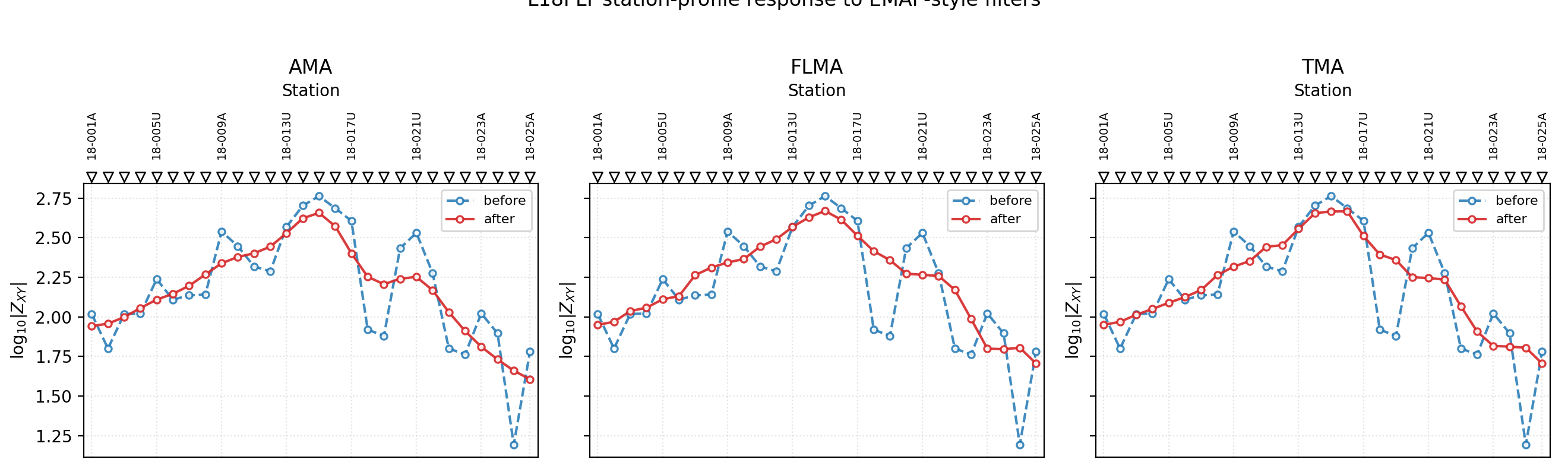
These filters assume that station order and station spacing are meaningful. They are most useful on survey lines where neighboring stations should share a broad geoelectric trend and sudden station-to-station jumps are likely to be static shift or local noise. They are less appropriate when a sharp station-local feature is a known target.

EMAP Reports And Plots

Before using an EMAP-filtered survey downstream, summarize where the filter changed the data.

import matplotlib.pyplot as plt

from pycsamt.emtools import (
    apply_emap_filter,
    emap_filter_report,
    ensure_sites,
    plot_emap_filter_profile,
    plot_emap_filter_psection,
)

sites = ensure_sites("data/AMT/WILLY_DATA/L18PLT", recursive=True)
flma = apply_emap_filter(
    sites,
    method="flma",
    window=5,
    component="xy",
    inplace=False,
)

report = emap_filter_report(
    sites,
    flma,
    component="xy",
)
print(report.sort_values("rms_delta_log10_abs_z", ascending=False).head())

fig, ax = plt.subplots(figsize=(8, 4))
plot_emap_filter_profile(
    sites,
    flma,
    method="flma",
    component="xy",
    ax=ax,
)
fig.tight_layout()
fig.savefig("emap_filter_profile_xy.png", dpi=200)
plt.close(fig)

fig = plot_emap_filter_psection(
    sites,
    flma,
    method="flma",
    component="xy",
)
fig.savefig("emap_filter_psection_xy.png", dpi=200)
plt.close(fig)

    station component  ...  median_delta_log10_abs_z  rms_delta_log10_abs_z
18  18-019U        xy  ...                  0.415765               0.505929
26  18-024U        xy  ...                  0.346431               0.401617
22  18-022U        xy  ...                  0.360391               0.391346
17  18-018A        xy  ...                  0.361853               0.377488
23  18-022V        xy  ...                  0.300769               0.310826

[5 rows x 5 columns]

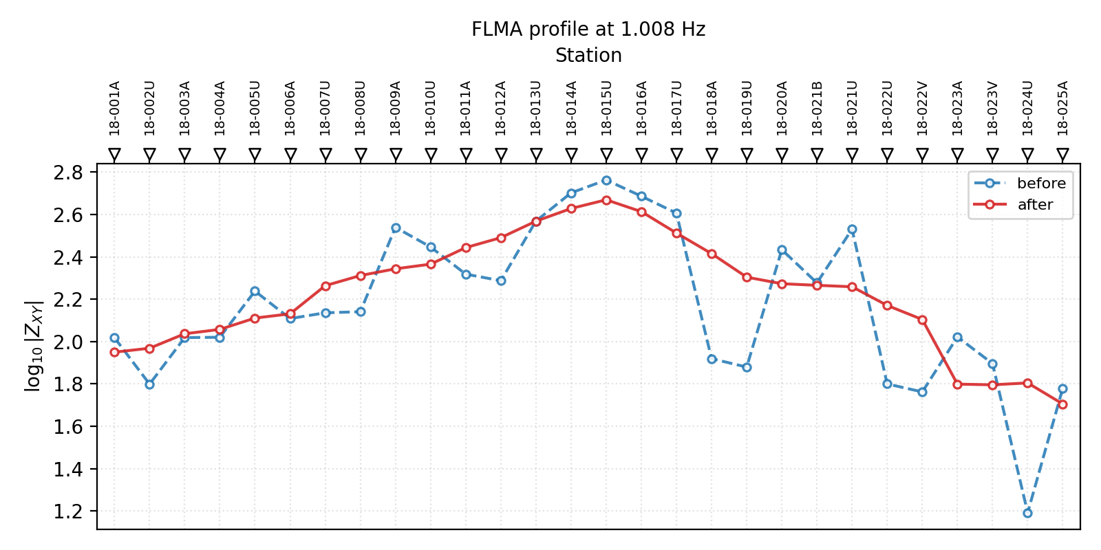
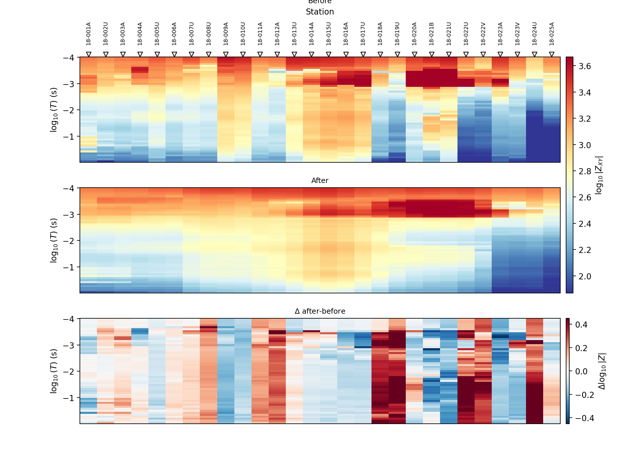
plot_emap_filter_profile is the quickest way to check one frequency profile along the line. plot_emap_filter_psection shows the before/after/delta pseudo-section across stations and periods. Use both: one exposes station-to-station behavior clearly, and the other shows whether corrections concentrate in a narrow period band.

Confidence-Gated EMAP Filtering

confidence_gated_emap_filter connects the noise-removal module to the QC module. It builds a frequency confidence table, computes an EMAP filtered candidate, then decides row by row how much filtered data to use:

• confidence above ci_hi: preserve the original row;

• confidence below ci_lo: use the filtered row;

• confidence between the thresholds: blend original and filtered rows.

from pycsamt.emtools import confidence_gated_emap_filter, ensure_sites

sites = ensure_sites("data/AMT/WILLY_DATA/L18PLT", recursive=True)

result = confidence_gated_emap_filter(
    sites,
    method="flma",
    window=5,
    ci_hi=0.90,
    ci_lo=0.50,
    component="xy",
)

print(result.summary())
print(result.report.head())
print(result.decisions.head())

gated_sites = result.sites

EMAPFilterResult(method='flma', confidence='composite', preserved=0, blended=1411, filtered=73)
   station  n_freq  ...  median_confidence  median_delta_log10_abs_z
0  18-001A      53  ...           0.711753                 -0.020918
1  18-002U      53  ...           0.749480                  0.015749
2  18-003A      53  ...           0.666613                  0.046988
3  18-004A      53  ...           0.735994                  0.004156
4  18-005U      53  ...           0.728841                 -0.025544

[5 rows x 8 columns]
   station  frequency_hz  period_s  ...  blend_weight   action  delta_log10_abs_z
0  18-001A       10400.0  0.000096  ...      0.109609  blended          -0.002075
1  18-001A        8707.0  0.000115  ...      0.134217  blended          -0.001228
2  18-001A        7289.0  0.000137  ...      0.142135  blended          -0.001559
3  18-001A        6102.0  0.000164  ...      0.236784  blended          -0.006566
4  18-001A        5108.0  0.000196  ...      0.437715  blended          -0.007875

[5 rows x 8 columns]

The return value is an EMAPFilterResult. It keeps the processed sites object, a station-level report, a row-level decisions table, the EMAP method, and the confidence thresholds. The convenience properties n_preserved, n_blended, and n_filtered are useful for logging.

from pycsamt.emtools import confidence_gated_emap_filter, ensure_sites

sites = ensure_sites("data/AMT/WILLY_DATA/L18PLT", recursive=True)
result = confidence_gated_emap_filter(sites, method="flma")

print(result.n_preserved)
print(result.n_blended)
print(result.n_filtered)

most_filtered = (
    result.report.sort_values(
        ["n_filtered", "median_confidence"],
        ascending=[False, True],
    )
    .loc[:, ["station", "n_preserved", "n_blended", "n_filtered", "median_confidence"]]
)
print(most_filtered.head(10))

0
1411
73
    station  n_preserved  n_blended  n_filtered  median_confidence
22  18-022U            0         38          15           0.569810
24  18-023A            0         41          12           0.612583
5   18-006A            0         47           6           0.764254
12  18-013U            0         48           5           0.669948
20  18-021B            0         49           4           0.594338
17  18-018A            0         50           3           0.585752
26  18-024U            0         50           3           0.631934
11  18-012A            0         50           3           0.651210
2   18-003A            0         50           3           0.666613
13  18-014A            0         50           3           0.699489

This is usually safer than applying the same spatial filter everywhere. High-confidence rows remain close to the measurement, while low confidence rows are allowed to borrow more from station-neighbor structure.

Full Pipeline

remove_noise_pipeline provides a compact chain for common cleaning: power-line notching, frequency smoothing, and optional group-trend shrinkage. It is convenient for batch processing, but you should still run the individual diagnostics first so you know which part of the pipeline is doing the work.

from pathlib import Path

from pycsamt.emtools import ensure_sites, remove_noise_pipeline

sites = ensure_sites("data/AMT/WILLY_DATA/L18PLT", recursive=True)

cleaned = remove_noise_pipeline(
    sites,
    mains_hz=50.0,
    n_harm=30,
    tol_hz=0.08,
    notch_mode="interp",
    smooth_win=5,
    smooth_kind="tri",
    gate_snr=2.5,
    group_shrink=False,
    inplace=False,
)

output_dir = Path("outputs/remove_noise")
output_dir.mkdir(parents=True, exist_ok=True)

The exact keyword names are intentionally close to the lower-level functions. Keep your pipeline call in a script or notebook with all parameters written out. That makes the processing reproducible and prevents hidden defaults from changing the interpretation later.

QC Figures For Noise Removal

The dedicated nr_qc_* figures compare a raw survey with a named noise-removal method. They are designed to be used after a method is chosen, not as a substitute for choosing the method carefully.

import matplotlib.pyplot as plt

from pycsamt.emtools import (
    ensure_sites,
    nr_qc_delta_offdiag_psection,
    nr_qc_harmonic_waterfall,
    nr_qc_snr_gain_profile,
    nr_qc_station_offdiag_curves,
)

sites = ensure_sites("data/AMT/WILLY_DATA/L18PLT", recursive=True)

fig, ax = plt.subplots(figsize=(9, 5))
nr_qc_delta_offdiag_psection(
    sites,
    method="pipeline",
    ax=ax,
)
fig.savefig("nr_qc_delta_offdiag_psection.png", dpi=200)
plt.close(fig)

fig, ax = plt.subplots(figsize=(8, 4))
nr_qc_snr_gain_profile(
    sites,
    method="pipeline",
    ax=ax,
)
fig.tight_layout()
fig.savefig("nr_qc_snr_gain_profile.png", dpi=200)
plt.close(fig)

fig, ax = plt.subplots(figsize=(9, 5))
nr_qc_harmonic_waterfall(
    sites,
    method="notch",
    mains_hz=50.0,
    n_harm=5,
    tol_hz=25.0,
    ax=ax,
)
fig.savefig("nr_qc_harmonic_waterfall.png", dpi=200)
plt.close(fig)

fig, ax = plt.subplots(figsize=(8, 4))
nr_qc_station_offdiag_curves(
    sites,
    method="pipeline",
    station="18-016A",
    ax=ax,
)
fig.tight_layout()
fig.savefig("nr_qc_station_offdiag_curves_18-016A.png", dpi=200)
plt.close(fig)

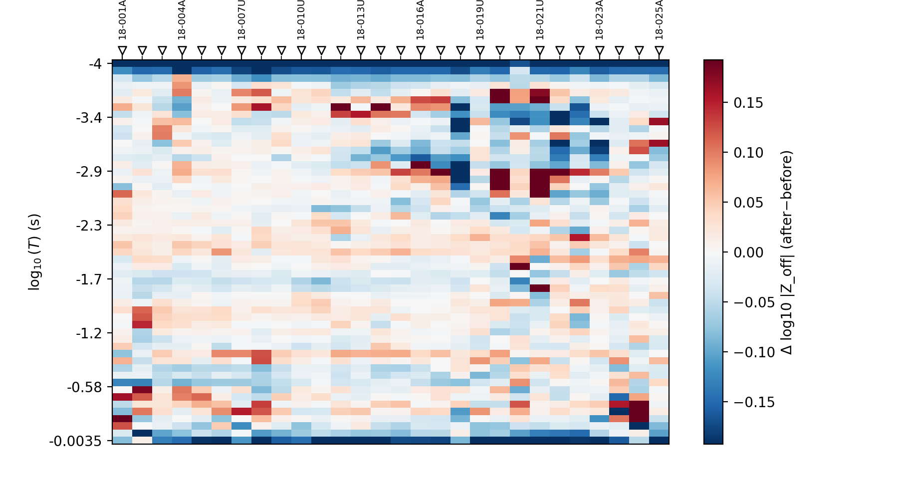
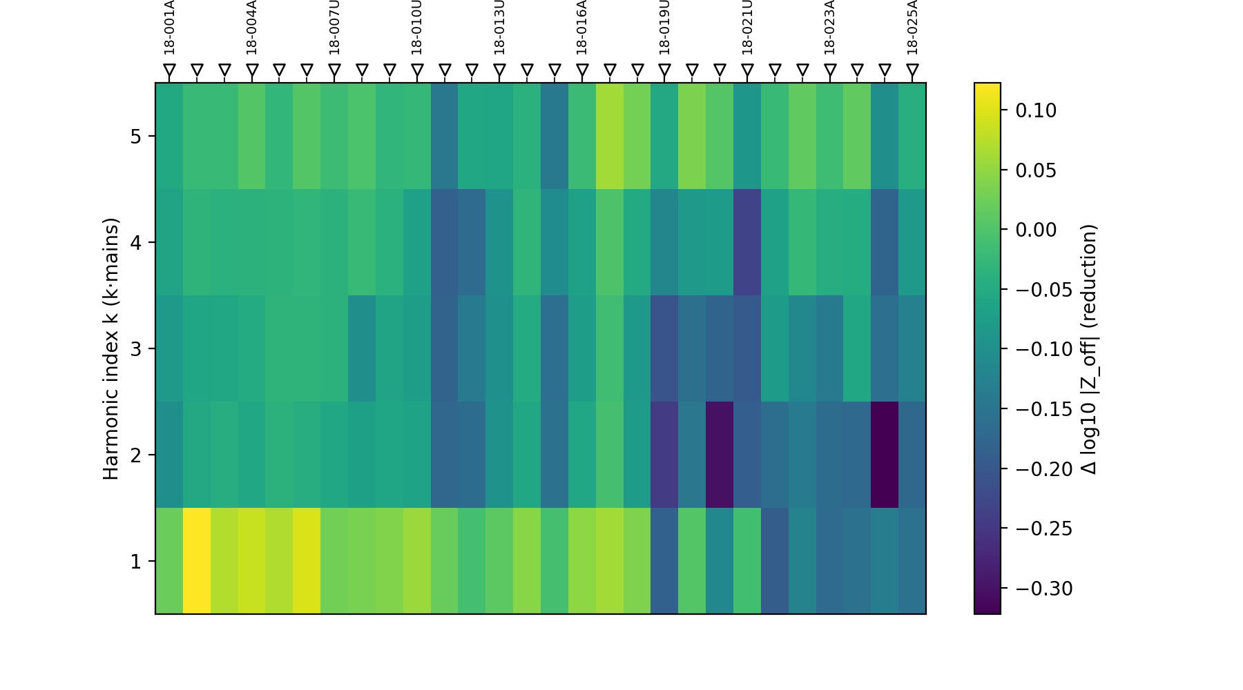
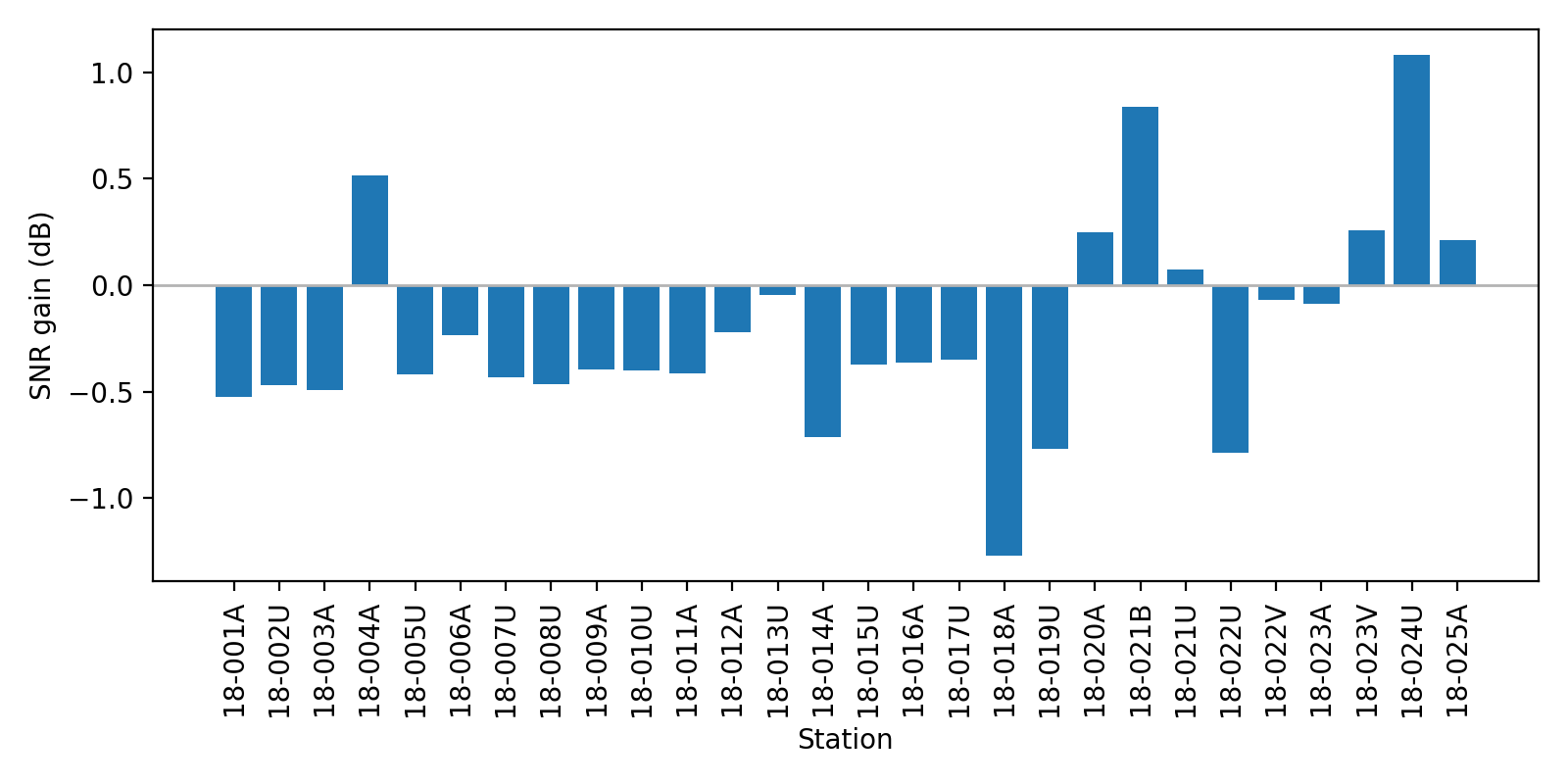
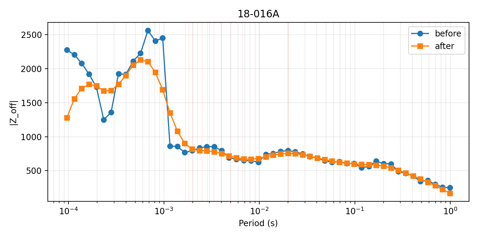
nr_qc_delta_offdiag_psection shows where off-diagonal magnitude changed in station-period space. nr_qc_snr_gain_profile summarizes SNR gain by station. nr_qc_harmonic_waterfall is specific to power-line harmonic reduction. nr_qc_station_offdiag_curves is the plainest check: one station, before and after, on the same axes.

Choosing A Treatment

Start with the least interpretive operation that addresses the observed problem.

• If only known harmonic rows are contaminated, start with notch_powerline.

• If curves are locally jagged but geologically plausible, try smooth_logfreq with a small window.

• If the whole curve should be smooth in apparent resistivity and phase, try smooth_rho_phase and inspect phase behavior.

• If one row is a spike, use hampel_filter_freq.

• If one station differs from its neighbors at the same frequencies, use spatial_median_filter or an EMAP filter.

• If many stations share a coherent trend but a few observations depart from it, test rpca_offdiag_denoise carefully.

• If QC confidence is already available, prefer confidence_gated_emap_filter over applying one fixed-strength spatial filter everywhere.

Do not stack every function by default. Each step changes the transfer function. A defensible workflow has a diagnostic reason for every correction and a before/after figure showing the effect.

Reproducible Bundle

A practical processing bundle usually contains four outputs:

from pathlib import Path

import matplotlib.pyplot as plt

from pycsamt.emtools import (
    ensure_sites,
    nr_qc_station_offdiag_curves,
    remove_noise_pipeline,
)
from pycsamt.emtools.remove_noise import emi_mitigation_report, snr_table

out = Path("outputs/remove_noise_l18plt")
out.mkdir(parents=True, exist_ok=True)

sites = ensure_sites("data/AMT/WILLY_DATA/L18PLT", recursive=True)

snr_table(sites).to_csv(out / "snr_table_raw.csv", index=False)
emi_mitigation_report(
    sites,
    remote_reference_attempted=False,
    mains_hz=50.0,
    n_harm=30,
    tol_hz=0.08,
    notch_mode="interp",
).to_csv(out / "emi_mitigation_report.csv", index=False)

cleaned = remove_noise_pipeline(
    sites,
    mains_hz=50.0,
    notch_mode="interp",
    smooth_win=5,
    smooth_kind="tri",
    gate_snr=2.5,
    group_shrink=False,
    inplace=False,
)

fig, ax = plt.subplots(figsize=(8, 4))

nr_qc_station_offdiag_curves(
    sites,
    method="pipeline",
    station="18-016A",
    ax=ax,
)
fig.savefig(out / "station_18-016A_pipeline_offdiag.png", dpi=200)
plt.close(fig)

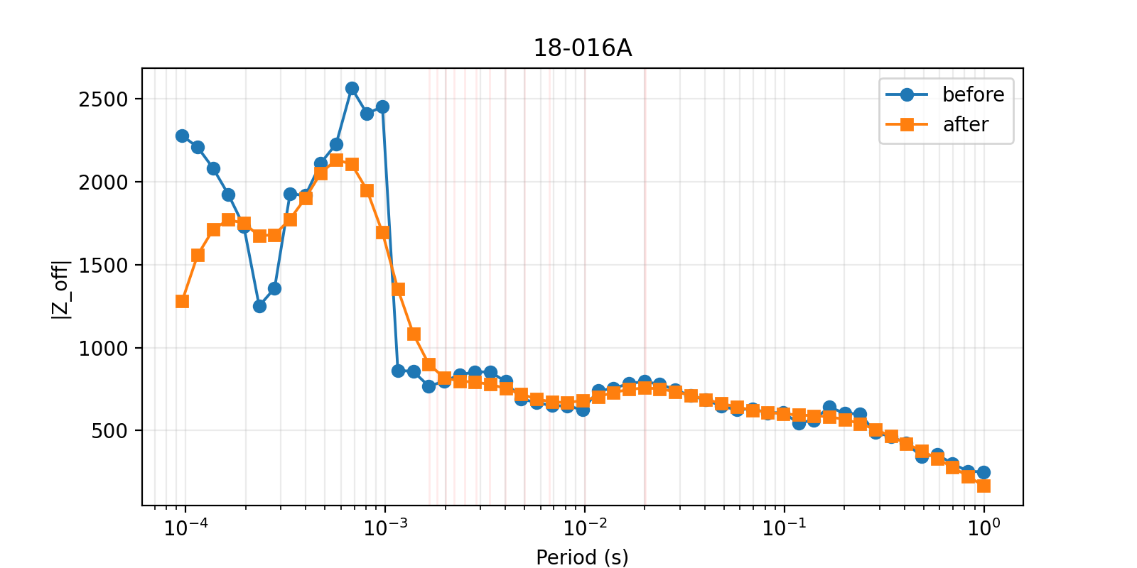
Keep the raw SNR table, EMI report, processing script, and representative QC figures together. That gives reviewers enough information to understand both the data quality and the editing decisions.

Worked Example

The example uses the real L18PLT survey where possible and small synthetic dense-frequency objects only where the real frequency grid does not contain power-line harmonic rows. It demonstrates SNR diagnostics, notching, smoothing, Hampel/spatial/RPCA denoising, consistency enforcement, masking, group-trend shrinkage, EMAP filtering, confidence-gated EMAP filtering, the full pipeline, and the dedicated QC plots.

Open the rendered gallery page here: Noise removal and spatial filtering (pycsamt.emtools.remove_noise).