16.9. Maxwell Adapters#

A MaxwellProblem or TriProblem is inert data: a mesh, a conductivity array, frequencies, receivers, and requested components. Something still has to turn that data into a forward response, and that something is a Maxwell adapter. Every concrete adapter in pycsamt.forward.maxwell – whether it wraps an in-repository finite-difference solver or shells out to a compiled external binary – inherits the same two-sided contract from BaseMaxwellAdapter: a preflight assessment of the problem against its declared backend capability, and a postflight validation of whatever the backend returns. Maxwell Forward Modelling and Solver Contracts derives why that boundary has to be this strict; this page stays at the level of “which adapter do I reach for, and what does calling it actually look like.”

16.9.1. Choosing An Adapter#

Five concrete adapters are shipped today. They fall into two families: three run entirely in-process against in-repository solvers, and two shell out to a compiled external executable that pyCSAMT does not bundle.

Adapter	Dimension	Components	Topography	Executable	Best for
`MT2DAdapter`	2-D	`zxy`, `zyx`	No	none (in-repo)	Quick, validated 2-D TE/TM prototyping and teaching.
`MT3DAdapter`	3-D	`zxx`, `zxy`, `zyx`, `zyy`	No	none (in-repo)	Small research-grid 3-D checks; not a production solver.
`TriFEM2DAdapter`	2-D	`zxy`, `zyx`	Yes	none (in-repo)	2-D forward modelling over real topography without an external build.
`ModEm3DAdapter`	3-D	`zxx`, `zxy`, `zyx`, `zyy`	No	`Mod3DMT` (ModEM)	Production-grade 3-D forward checks and training-data generation.
`Mare2DEMAdapter`	2-D	`zxy`, `zyx`	Yes	`MARE2DEM`	Production 2.5-D/CSEM forward modelling with topography.

Every row’s backend capability is a checkable claim, not a label taken on trust – Maxwell Backend Registry covers exactly what assess() checks and how a backend gets found by that declaration instead of by import; this page stays at the level of one call to adapter.solve(problem):

>>> from pycsamt.forward.maxwell.mt2d import MT2DAdapter
>>> capability = MT2DAdapter().capabilities
>>> capability.dimensions, capability.components
((2,), ('zxy', 'zyx'))
>>> capability.verified_benchmarks
('half-space', 'layered-earth')

verified_benchmarks is where the “Best for” column above actually comes from: an adapter that has not been checked against benchmarks (Maxwell Analytic Benchmarks) should be trusted no further than an unverified guess, regardless of how confident its dimensionality and component support look. The three in-repository adapters need nothing beyond pycsamt and NumPy/SciPy; the two external adapters additionally need a compiled executable, obtained the way Compiling the External Solvers describes. That split matters for scope, too: these adapters exist to produce a single validated forward response or a batch of them (Maxwell Caching And Batch Solving), not to run a full inversion project. Building a native ModEM or MARE2DEM project – meshes, covariance, iterative inversion, native file review – is the job of ModEM and MARE2DEM; reach for those pages once a forward check here has already told you the solver and geometry are worth committing to.

16.9.2. In-Repository 2-D Solve#

MT2DAdapter wraps the same finite-difference solver already introduced in Solvers And Grids (MT2DForward), but through the canonical contract instead of a bespoke Grid2D. Every receiver must sit exactly at the surface and the earth model has no inactive cells – both checked in assess before a solve is attempted, not discovered afterward:

>>> import numpy as np
>>> from pycsamt.forward.maxwell import MaxwellMesh, MaxwellProblem, ReceiverSet
>>> from pycsamt.forward.maxwell.mt2d import MT2DAdapter

>>> mesh = MaxwellMesh(np.linspace(0, 10_000, 41), np.linspace(0, 5_000, 31))
>>> problem = MaxwellProblem(
...     mesh, np.full(mesh.shape, 1.0 / 100.0), [10.0, 1.0],
...     ReceiverSet([[5_000.0, 0.0]], ["S00"]), ("zxy", "zyx"),
... )
>>> adapter = MT2DAdapter(verbose=False)
>>> result = adapter.solve(problem)
>>> result.shape
(1, 2, 2)
>>> result.backend_name, result.backend_version
('mt2d', '1.0')
>>> bool(np.all(result.diagnostics.converged))
True
>>> result.problem_hash == problem.problem_hash
True

The last line is postflight validation made visible: result carries the exact problem hash of the problem it was solved from ((13) in Maxwell Forward Modelling and Solver Contracts defines what goes into that hash), so a stored or later-compared result can always be tied back to the input that produced it. Moving a receiver off the surface is rejected before MT2DForward ever runs:

>>> buried = ReceiverSet([[5_000.0, 50.0]], ["S00"])
>>> bad_problem = MaxwellProblem(
...     mesh, np.full(mesh.shape, 1.0 / 100.0), [10.0, 1.0],
...     buried, ("zxy", "zyx"),
... )
>>> report = adapter.assess(bad_problem)
>>> report.compatible
False
>>> report.errors
('mt2d only evaluates receivers at the surface (z=0)',)
>>> adapter.solve(bad_problem)
Traceback (most recent call last):
...
pycsamt.forward.maxwell.adapters.IncompatibleProblemError: backend 'mt2d' is incompatible: mt2d only evaluates receivers at the surface (z=0)

A single receiver at 10 and 1 Hz is enough to exercise the contract, but not enough to see what a 2-D adapter is actually for: reading a lateral forward response across a profile. The executed study below sweeps twelve frequencies at seven stations straddling a shallow 5 ohm m conductor buried in a 100 ohm m background, using the same MT2DAdapter shown above:

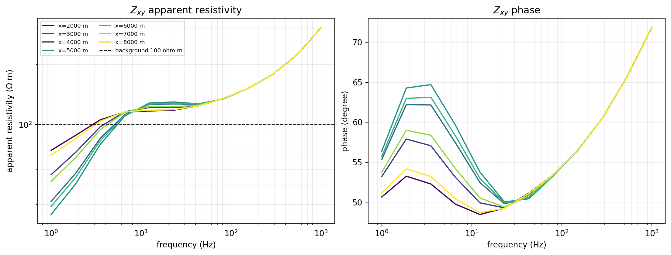
Apparent resistivity and phase from MT2DAdapter across seven stations over a shallow conductor. — Apparent resistivity and phase, (6), from `MT2DAdapter` for seven stations spanning a shallow 5 ohm m conductor.#

Every station’s apparent resistivity converges toward the 100 ohm m background at both ends of the swept band – the highest frequencies barely sense the conductor because their skin depth stays shallow, and the lowest frequencies average it into the surrounding half-space – while the mid-band curves dip and the phase rises above the 45-degree half-space value exactly where the stations sit closest to the conductor. That mid-band lift is the diagnostic signature a real 2-D survey is designed to resolve; seeing it appear from a validated adapter rather than a bespoke script is the point of routing this problem through MT2DAdapter instead of calling MT2DForward directly.

16.9.3. Research-Only 3-D Solve#

MT3DAdapter answers the natural next question – “what about a full 3-D earth” – but its capability declaration is explicit about the cost: a default 6,000-cell ceiling, because the direct sparse solve behind it does not scale to production mesh sizes. Raising max_cells changes computational risk, not numerical maturity, and it has no registration function in the backend registry (unlike the other four adapters), a deliberate reminder that it is meant to be reached for directly rather than discovered by capability search:

>>> from pycsamt.forward.maxwell.mt3d import MT3DAdapter

>>> mesh3d = MaxwellMesh(
...     np.linspace(0, 4_000, 9), np.linspace(0, 3_000, 11), np.linspace(0, 4_000, 9)
... )
>>> problem3d = MaxwellProblem(
...     mesh3d, np.full(mesh3d.shape, 1.0 / 100.0), [1.0],
...     ReceiverSet([[2_000.0, 2_000.0, 0.0]], ["S00"]), ("zxx", "zxy", "zyx", "zyy"),
... )
>>> mt3d_adapter = MT3DAdapter()
>>> mt3d_adapter.capabilities.maximum_cells
6000
>>> result3d = mt3d_adapter.solve(problem3d)
>>> result3d.shape
(1, 1, 4)
>>> np.round(result3d.impedance_v_a[0, 0, :], 4)
array([ 0.    +0.j    ,  0.0199+0.0211j, -0.0199-0.0211j,  0.    -0.j    ])

A single station at a single frequency is already enough to show what a correct 3-D half-space response looks like through this contract: the diagonal components zxx/zyy collapse to zero and the off-diagonal components are near-mirror images of each other, exactly as (5) predicts for a laterally uniform earth. There is little value in plotting a single complex number per component, so this section stops at the numbers – a figure earns its place only once a receiver profile or a heterogeneous model gives it something to show, which is precisely what the next two adapters provide without MT3DAdapter’s cell ceiling.

16.9.4. Topography-Aware Triangular FEM#

TriFEM2DAdapter is the only in-repository adapter that declares supports_topography=True. It solves on a TriMesh rather than a structured MaxwellMesh, and every receiver must coincide with an actual mesh node on the mesh’s own local surface – not z=0, but wherever that station’s terrain elevation puts it. build_graded_tri_mesh() builds such a mesh directly from a topography polyline, grading triangle size away from the receivers so the fine resolution needed near stations does not have to be paid for everywhere:

View TriFEM2DAdapter mesh-and-response source codeClick to inspect and copy the complete code

def make_trifem2d_mesh_response() -> tuple[int, tuple[int, int, int], bool]:
    station_x = np.linspace(-800, 800, 9)
    topo_x = np.linspace(-1200, 1200, 9)
    topo_z = -60 * np.exp(-((topo_x / 500) ** 2))
    mesh = build_graded_tri_mesh(
        (-1200, 1200), (0, 2500), station_x,
        surface_cell_m=30, growth_rate=1.35,
        topo_x_m=topo_x, topo_z_m=topo_z,
    )
    centroid_z = mesh.nodes_m[mesh.triangles, 1].mean(axis=1)
    resistivity_ohm_m = np.where(centroid_z < 150.0, 20.0, 300.0)
    receiver_z = np.interp(station_x, topo_x, topo_z)
    receivers = ReceiverSet(
        np.column_stack([station_x, receiver_z]),
        [f"S{i:02d}" for i in range(len(station_x))],
    )
    problem = TriProblem(mesh, 1.0 / resistivity_ohm_m, [200.0, 20.0], receivers)
    result = TriFEM2DAdapter().solve(problem)

    fig, axes = plt.subplots(1, 2, figsize=(12, 4.6), constrained_layout=True)
    triangulation = plt.matplotlib.tri.Triangulation(
        mesh.nodes_m[:, 0], mesh.nodes_m[:, 1], mesh.triangles
    )
    im = axes[0].tripcolor(triangulation, facecolors=resistivity_ohm_m,
                            cmap="turbo_r", vmin=20, vmax=300, edgecolors="white",
                            linewidth=0.15)
    axes[0].plot(topo_x, topo_z, color="black", lw=1.5)
    axes[0].scatter(station_x, receiver_z, marker="v", color="black", s=36, zorder=5)
    axes[0].set_ylim(600, -100)
    axes[0].set(title="Graded triangular mesh on real topography",
                xlabel="x (m)", ylabel="z (m)")
    fig.colorbar(im, ax=axes[0], label=r"resistivity ($\Omega$ m)")

    for ci, label in enumerate(("zxy", "zyx")):
        rhoa, _ = _rhoa_phase(result.impedance_v_a[:, 0, ci], result.frequencies_hz[0])
        axes[1].plot(station_x, rhoa, marker="o", label=f"{label}, 200 Hz")
    for ci, label in enumerate(("zxy", "zyx")):
        rhoa, _ = _rhoa_phase(result.impedance_v_a[:, 1, ci], result.frequencies_hz[1])
        axes[1].plot(station_x, rhoa, marker="s", ls="--", label=f"{label}, 20 Hz")
    axes[1].set(title="Apparent resistivity at each receiver",
                xlabel="station x (m)", ylabel=r"apparent resistivity ($\Omega$ m)")
    axes[1].legend(fontsize=8)
    axes[1].grid(alpha=.25)
    _save(fig, "maxwell_adapters_trifem2d_mesh_response.png")
    return mesh.n_triangles, result.shape, bool(np.all(result.diagnostics.converged))

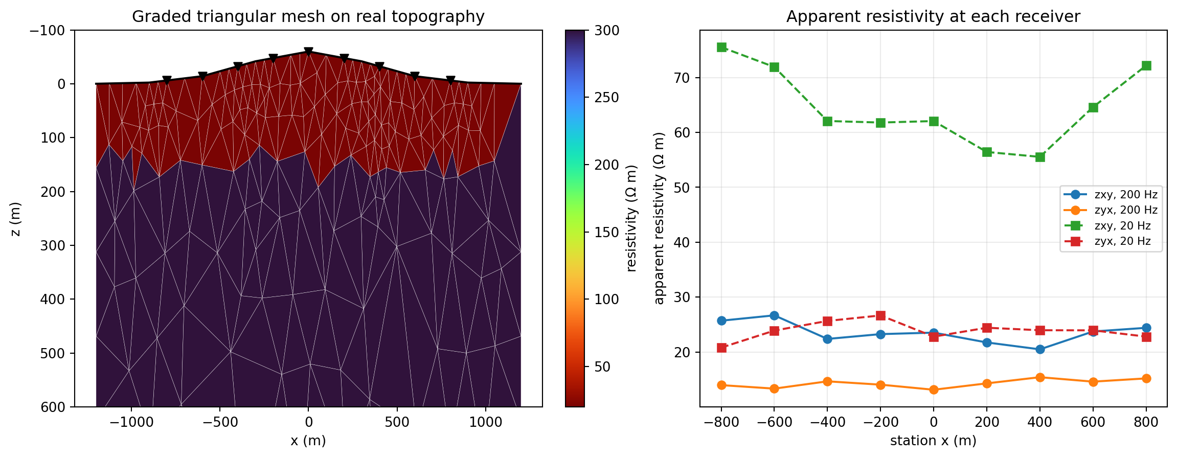
Graded triangular mesh following real topography, and apparent resistivity from TriFEM2DAdapter at each receiver. — A 384-triangle graded mesh following a synthetic ridge, and the apparent-resistivity response `TriFEM2DAdapter` returns at each receiver for two frequencies.#

The mesh panel is the more important half of this figure. Triangle density follows the receivers (dense under the ridge crest, coarse toward the padded sides and at depth) and the conductive near-surface layer – 20 ohm m against a 300 ohm m background – is carried on the triangulation exactly as it sits under the terrain, not projected onto a flat datum. The response panel then shows what topography does to a 2-D adapter that a flat-surface adapter cannot represent at all: the 20 Hz curves swing by roughly 20 ohm m across nine stations sitting on the same two-layer earth, purely from elevation and local slope, while the higher-frequency 200 Hz curves – shallower skin depth, less sensitive to the broad ridge shape – stay comparatively flat. Running the same receivers through MT2DAdapter is not an option here; that adapter’s own preflight rejects anything off z=0, which is exactly the check exercised earlier in this page.

16.9.5. External Solver Adapters#

ModEm3DAdapter and Mare2DEMAdapter both subclass BaseExternalMaxwellAdapter instead of BaseMaxwellAdapter directly: on top of the usual preflight/postflight pair, they resolve an executable, write native input files into an isolated run directory, launch the process under a timeout policy, and parse its native output back into the same ForwardResult contract every other adapter returns. Maxwell Forward Modelling and Solver Contracts covers that lifecycle in full; the practical consequence here is that availability of an executable, compatibility of a problem, and validity of a result are three independent things, and this contract checks all three separately rather than assuming one implies the others.

Resolving a missing executable fails loudly rather than silently returning an empty result:

>>> from pycsamt.forward.maxwell.external import ExecutableNotFoundError, resolve_executable
>>> resolve_executable("does-not-exist-xyz")
Traceback (most recent call last):
...
pycsamt.forward.maxwell.external.ExecutableNotFoundError: executable 'does-not-exist-xyz' was not found on PATH or in ().

Both adapters can always be constructed and their capabilities inspected without any executable at all – an external adapter declares its scope the same way an in-repository one does, before it ever needs to find a binary:

>>> from pycsamt.forward.maxwell import ExternalRunPolicy
>>> from pycsamt.forward.maxwell.modem3d import ModEm3DAdapter
>>> from pycsamt.forward.maxwell.mare2dem import Mare2DEMAdapter
>>> ModEm3DAdapter(run_policy=ExternalRunPolicy("does-not-exist-xyz")).capabilities.name
'modem3d'
>>> mare_capability = Mare2DEMAdapter(
...     run_policy=ExternalRunPolicy("does-not-exist-xyz")
... ).capabilities
>>> mare_capability.supports_topography
True
>>> mare_capability.verified_benchmarks
()

That last, empty tuple is worth pausing on: this pycsamt release ships Mare2DEMAdapter without any verified benchmark recorded in its capability declaration, even though a real compiled-MARE2DEM benchmark exists in pycsamt’s own test suite and the real-binary validation behind MARE2DEM used the same adapter architecture. Until that declaration is updated, treat Mare2DEMAdapter as architecturally complete but not yet self-certifying through this contract – exactly the gap verified_benchmarks exists to expose rather than paper over. Whether an executable can even be found is a separate, environment-specific question, checked by registering both backends and asking the registry rather than either adapter directly:

>>> from pycsamt.forward.maxwell import register_mt2d_backend, list_backends
>>> from pycsamt.forward.maxwell.tri_fem2d import register_trifem2d_backend
>>> from pycsamt.forward.maxwell.modem3d import register_modem3d_backend
>>> from pycsamt.forward.maxwell.mare2dem import register_mare2dem_backend
>>> register_mt2d_backend(replace=True)
>>> register_trifem2d_backend(replace=True)
>>> register_modem3d_backend(replace=True)
>>> register_mare2dem_backend(replace=True)
>>> {name: info["available"] for name, info in list_backends().items()}
{'mt2d': True, 'trifem2d': True, 'modem3d': True, 'mare2dem': False}
>>> list_backends()["mare2dem"]["reason"]
"executable 'mpirun' was not found on PATH or in ()."

The two in-repository adapters are trivially “available” because they need nothing beyond pycsamt itself. modem3d reads True on the machine that built this page because a compiled Mod3DMT happens to sit in pycsamt’s vendored ModEM source tree; mare2dem reads False because its default Mare2DEMConfig looks for an mpirun launcher that is not installed here – not because MARE2DEM itself is unreachable, which is exactly the kind of distinction the reason string exists to preserve instead of collapsing into a bare False. Compiling the External Solvers covers building both solvers from source.

A compiled Mod3DMT being available means ModEm3DAdapter can run for real here, against the same kind of calibrated, unpadded mesh pycsamt’s own real-binary tests use – ModEM synthesizes its own air layers, so this mesh only needs to describe the earth:

>>> n, h = 8, 300.0
>>> modem_mesh = MaxwellMesh(np.arange(n + 1) * h, np.arange(11) * h, np.arange(n + 1) * h)
>>> modem_receivers = ReceiverSet([[n * h / 2, n * h / 2, 0.0]], ["S00"])
>>> modem_problem = MaxwellProblem(
...     modem_mesh, np.full(modem_mesh.shape, 1.0 / 100.0), [1.0, 0.5],
...     modem_receivers, ("zxx", "zxy", "zyx", "zyy"),
... )
>>> modem_adapter = ModEm3DAdapter()
>>> modem_result = modem_adapter.solve(modem_problem)
>>> modem_result.shape
(1, 2, 4)
>>> modem_result.backend_version
'modem-v6.2.6-adapter-1.0'
>>> mu0 = 4e-7 * np.pi
>>> rhoa_zxy = np.abs(modem_result.impedance_v_a[0, :, 1]) ** 2 / (mu0 * 2 * np.pi * modem_result.frequencies_hz)
>>> np.round(rhoa_zxy, 2)
array([103.08, 102.16])

103 and 102 ohm m recovered from a real compiled ModEM run of a true 100 ohm m half-space, on a mesh of only 640 earth cells, is a genuinely useful sanity check before trusting a much larger production run. The same adapter also passes pycsamt’s analytic layered-earth benchmark within its default thresholds – a 100/30/500 ohm m three-layer earth solved on this machine’s Mod3DMT comes back with a normalized RMS error of 0.0144, a worst-case amplitude error of 1.3%, and a worst-case phase error of 0.41 degree, all measured against layered_earth_impedance()’s closed-form recurrence – the frequency-dependent counterpart to the plain half-space case in (16) – rather than against another numerical solver. Maxwell Analytic Benchmarks covers how that comparison, and the acceptance thresholds behind outcome.passed, are built.

16.9.6. Common Mistakes#

Passing mark_air_inactive=True into an incompatible adapter: to_problem() can mark air cells inactive, but none of the five adapters on this page declare supports_inactive_cells=True. Preflight will reject the problem; the fix is to build the problem with inactive marking off, not to look for a workaround inside the adapter.
Assuming dimensionality support means validated: BackendCapabilities.dimensions says what shapes of problem an adapter will attempt. Only verified_benchmarks says what it has been checked against – and, as Mare2DEMAdapter shows above, those two lists can legitimately disagree within a single release.
Treating an unavailable registry entry as an incompatible problem: list_backends()[...]["available"] reports whether an executable was found, not whether a given problem would pass that backend’s assess. A missing binary and an unsupported problem raise through completely different paths – ExecutableNotFoundError versus IncompatibleProblemError – and conflating them in a script’s error handling hides which one actually happened.
Forgetting replace=True when swapping a registration: Registration is process-wide and silent by default: register_mt2d_backend() a second time without replace=True raises rather than quietly overwriting the first registration, which is deliberate in a long-running experiment where a silent solver swap could change numerical behaviour mid-run.
Trusting a station-level result MT2DAdapter reports as valid: The finite-difference solver behind MT2DAdapter falls back to 0 + 0j at a station with a near-zero surface magnetic field instead of raising, and a finite 0 + 0j passes the default validity check. A response that is suspiciously exactly zero at one station is worth inspecting directly rather than trusting result.valid alone.

16.9.7. Next Pages#

Maxwell Analytic Benchmarks shows how verified_benchmarks claims like the ones inspected on this page are actually produced and scored, including the layered-earth check just run against ModEm3DAdapter. Maxwell Caching And Batch Solving then covers running many problems through one of these adapters reliably, with retries and a resumable failure record.