6.2.5. Occam2D

pycsamt.models.occam2d provides the pyCSAMT interface to an Occam2DMT-style smooth 2-D inversion workflow. It prepares native input files, can run the external Fortran executable, loads iteration and response outputs, and provides plotting helpers for models, responses, pseudosections, misfit curves, station-level residuals, and 1-D station extracts.

Occam inversion is deliberately conservative. It seeks the smoothest model that fits the data to an acceptable normalized RMS misfit. For a residual vector \(r\), the usual RMS diagnostic is

\[\mathrm{RMS} = \sqrt{\frac{1}{N}\sum_{i=1}^{N} r_i^2}.\]

Occam iteration files store model parameters as log10 resistivity, \(m = \log_{10}(\rho)\). pyCSAMT preserves that convention in InversionResult.rho_2d and converts to physical resistivity only when a plot or downstream calculation needs it.

6.2.5.1. When To Use Occam2D

Occam2D is a good first production engine when:

• stations follow a profile and can be represented by 2-D geometry;

• the dominant resistivity structure is expected to be approximately 2-D;

• a smooth model is scientifically appropriate;

• TE/TM apparent resistivity and phase are the primary inversion data;

• the deliverable must include native files: Occam data, mesh, model, startup, iteration, response, and log files;

• the interpreter wants a reproducible external-code workflow rather than only an in-memory inversion result.

Occam2D is not a blocky geology engine. A sharp geological contact may appear as a smooth gradient because the regularization intentionally spreads structure unless the data require a sharper transition.

6.2.5.2. Package Map

The Occam2D package is organized around the native inversion lifecycle.

Area	Main objects	Purpose
Configuration	OccamConfig	Stores data selection, error floors, mesh options, startup controls, file names, and binary discovery name.
Input construction	InputBuilder	Builds data, mesh, model, and startup files from a survey source.
Native data	OccamData	Reads/writes Occam data files and builds data rows from EDI/Sites-like sources.
Mesh and model	OccamMesh, OccamModel	Build/read finite-element mesh geometry and the model-parameter mapping.
Startup and iterations	OccamStartup, OccamIter	Represent the iteration-zero startup file and non-zero iteration output files.
Execution	OccamRunner	Finds or compiles the executable, patches startup controls when requested, launches the solver, and captures stdout/stderr logs.
Results	InversionResult	Scans a completed run, loads mesh/model/data/log/iteration/response files, reconstructs rho_2d, and exports iter2dat.
Diagnostics	OccamResponse, OccamLog	Parse response residuals and convergence history.
Plotting	PlotModel, PlotResponse, PlotPseudo, PlotMisfit, PlotSounding1D, PlotSiteMisfit, PlotResponseGrid, PlotStation1DFit	Visual QC and interpretation views.
Validation	detect_file_type and is_* helpers	Recognize data, mesh, model, startup, iteration, response, and log files.

6.2.5.3. Configuration

OccamConfig is the source-of-truth object for a native Occam2D run. It can be created in Python, written to a configuration file template, edited, and loaded again.

>>> from pycsamt.models.occam2d import OccamConfig

>>> cfg = OccamConfig(
...     modes=["TE", "TM"],
...     error_floor_rho=0.05,
...     error_floor_phase=0.5,
...     freq_min=0.1,
...     freq_max=1000.0,
...     n_layers=36,
...     n_airlayers=5,
...     cell_size_horizontal=75.0,
...     cell_size_vertical_top=10.0,
...     depth_scale=1.18,
...     n_padding_x=8,
...     max_iterations=80,
...     target_misfit=1.0,
...     initial_rho=100.0,
...     data_file="OccamDataFile.dat",
...     mesh_file="Occam2DMesh",
...     model_file="Occam2DModel",
...     startup_file="Startup",
...     binary_name="Occam2D",
... )

>>> cfg.to_template("runs/profile_a_occam2d_v01/occam2d.yml")
>>> loaded = OccamConfig.from_file("runs/profile_a_occam2d_v01/occam2d.yml")
>>> print(loaded.modes, loaded.n_layers, loaded.cell_size_horizontal, loaded.target_misfit)
['TE', 'TM'] 36 75.0 1.0

The configuration groups four concerns.

Concern	Fields	Meaning
Data selection	modes, error_floor_rho, error_floor_phase, freq_min, freq_max	Which data rows are written and how minimum uncertainties are enforced.
Mesh geometry	n_layers, n_airlayers, cell_size_horizontal, cell_size_vertical_top, depth_scale, n_padding_x	Finite-element discretization near stations, at depth, and near lateral boundaries.
Startup controls	max_iterations, target_misfit, roughness_type, diagonal_penalties, stepsize_cut_count, debug_level, initial_rho, lagrange_start	Values written to the startup file, including the initial Lagrange multiplier (lagrange_start) and how many times its step size may be cut during one iteration’s line search (stepsize_cut_count).
Files and binary	data_file, mesh_file, model_file, startup_file, binary_name	Native file names inside the run directory and executable name used by the runner.

Use strict loading for project work. Unknown keys usually mean spelling mistakes or stale configuration files.

>>> from pycsamt.models.occam2d import OccamConfig

>>> cfg = OccamConfig.from_file("runs/profile_a_occam2d_v01/occam2d.yml")

>>> # old_occam2d.yml is the same file with one retired key appended:
>>> # "convergence_tol: 0.001"
>>> try:
...     OccamConfig.from_file("runs/profile_a_occam2d_v01/old_occam2d.yml")
... except ValueError as exc:
...     print(exc)
Unknown configuration parameter(s): convergence_tol

>>> # Migration only: ignore retired or unknown keys while cleaning old files.
>>> migrated = OccamConfig.from_file(
...     "runs/profile_a_occam2d_v01/old_occam2d.yml",
...     strict=False,
... )
>>> print(cfg.n_layers, migrated.n_layers)
36 36

strict=False does not fall back to defaults for the whole file – it drops only the keys the current OccamConfig no longer defines (convergence_tol here) and keeps every other value exactly as written, so migrated.n_layers still comes back as the 36 that was actually saved. strict=True on the same file refuses to guess and raises instead, which is what makes it the right default for everyday project work: a misspelled key fails loudly rather than silently reverting that one field to its OccamConfig default.

6.2.5.4. Native Files

Occam2D projects should be archived as native file sets. The final image alone is not enough to reproduce the inversion.

File	Object	Role
OccamDataFile.dat	OccamData	Observed data rows, station names, offsets, frequencies, Occam type codes, datum values, and uncertainties.
Occam2DMesh	OccamMesh	Finite-element mesh geometry, including air layers, earth layers, horizontal cells, and padding cells.
Occam2DModel	OccamModel	Mapping from mesh cells to inversion parameters.
Startup	OccamStartup	Startup file: data/model/mesh names, target misfit, iteration controls, starting parameters.
*.iter	OccamIter	Iteration files containing log10-resistivity parameter values and iteration diagnostics.
*.resp	OccamResponse	Response file: modeled responses and residual information for an iteration.
*.logfile or LogFile*	OccamLog	Convergence history and run-level diagnostic messages.
occam_stdout.log and occam_stderr.log	OccamRunner	Captured process streams from pyCSAMT-launched runs.

The validation helpers can classify files when scanning a run directory. They key off content, not extension, so a renamed file is still recognized correctly:

>>> from pycsamt.models.occam2d.validation import detect_file_type

>>> for path in [
...     "data/occam2D/OccamDataFile.dat",
...     "data/occam2D/Occam2DMesh",
...     "data/occam2D/Startup",
... ]:
...     print(path, detect_file_type(path))
data/occam2D/OccamDataFile.dat data
data/occam2D/Occam2DMesh mesh
data/occam2D/Startup startup

6.2.5.5. Build Input Files

InputBuilder constructs the four files required before an external Occam2D run can start. It consumes a Sites container, not a bare directory string, so a survey source is normalized once, up front, with from_any().

>>> from pycsamt.models.occam2d import InputBuilder, OccamConfig
>>> from pycsamt.site import Sites

>>> sites = Sites.from_any("data/AMT/WILLY_DATA/L18PLT")

>>> cfg = OccamConfig(
...     modes=["TE", "TM"],
...     freq_min=0.1,
...     freq_max=1000.0,
...     error_floor_rho=0.05,
...     error_floor_phase=0.5,
...     n_layers=32,
...     target_misfit=1.0,
... )

>>> builder = InputBuilder(
...     sites,
...     workdir="runs/profile_a_occam2d_v01/native",
...     config=cfg,
...     verbose=1,
... )
>>> builder.build(title="Profile A Occam2D inversion")

>>> print(builder.summary())
InputBuilder summary
  workdir   : runs/profile_a_occam2d_v01/native
  sites     : 28
  freqs     : 39
  data pts  : 4368
  mesh      : 42 x 37 cells
  params    : 512
  modes     : ['TE', 'TM']

The build chain is fixed:

1. OccamData.from_edi converts the survey source into Occam data rows.

2. OccamMesh.from_data builds a mesh from station offsets and mesh options.

3. OccamModel.from_mesh maps mesh cells to inversion parameters.

4. OccamStartup.from_model writes the initial parameter vector and run controls.

One-shot overrides passed to build update the stored configuration before files are written.

>>> builder.build(
...     modes=["TM"],
...     n_layers=40,
...     cell_size=50.0,
...     error_floor_rho=0.07,
...     freq_min=0.2,
...     freq_max=500.0,
...     title="Profile A TM-only sensitivity run",
... )
>>> print(builder.summary())
InputBuilder summary
  workdir   : runs/profile_a_occam2d_v01/native
  sites     : 28
  freqs     : 35
  data pts  : 1960
  mesh      : 66 x 45 cells
  params    : 1120
  modes     : ['TM']

Narrowing the frequency band and switching to a single mode roughly halved the data count (4368 to 1960), and the finer 50 m cell size more than doubled the mesh (42x37 to 66x45 cells) and free parameters (512 to 1120). Because these overrides persist on builder.config, write the resulting configuration to the run directory if this build is the one that gets kept.

6.2.5.6. Data Rows And Type Codes

Occam2D data files written by pyCSAMT use TE/TM apparent resistivity and phase rows, distinguished by type code:

• "TE" selects the \(Z_{xy}\) component, written as type codes 1 (\(\rho_a\)) and 2 (phase);

• "TM" selects the \(Z_{yx}\) component, written as type codes 5 (\(\rho_a\)) and 6 (phase);

• apparent resistivity is stored as \(\log_{10}(\rho_a)\);

• phase is stored in degrees;

• error_floor_rho is relative, for example 0.05 for five percent;

• error_floor_phase is absolute, in degrees.

Inspect the data object before running – this reads back the TM-only file just written above.

>>> from pycsamt.models.occam2d import OccamData

>>> data = OccamData.read("runs/profile_a_occam2d_v01/native/OccamDataFile.dat")

>>> print(data.n_sites, data.n_frequencies, data.n_data)
28 35 1960
>>> print(data.sites[:5])
['18-025A', '18-024U', '18-023V', '18-023A', '18-022V']
>>> print(data.offsets[:5])
[-2403.  -2297.8 -2201.6 -2199.7 -2101.7]

Station order and offsets matter because the mesh and pseudosections are built around that profile geometry – notice the offsets are already sorted by chainage, not by the original EDI file order.

6.2.5.7. Mesh And Model Review

The mesh and model determine what kind of smoothness the inversion can express. Before launching a long external run, inspect:

• horizontal cell width near stations;

• number of padding cells on each side;

• top cell thickness and depth growth factor;

• number of air layers and earth layers;

• total number of model parameters;

• whether the mesh is far wider and deeper than the interpreted target.

>>> from pycsamt.models.occam2d import OccamMesh, OccamModel

>>> mesh = OccamMesh.read("runs/profile_a_occam2d_v01/native/Occam2DMesh")
>>> model = OccamModel.read("runs/profile_a_occam2d_v01/native/Occam2DModel")

>>> print(mesh.n_xcells, mesh.n_zcells)
66 45
>>> print(model.n_params)
1120

Fine cells can improve near-surface representation, but they also increase runtime and may exaggerate the apparent resolution of poorly constrained structure. Padding moves boundaries away from the profile but also increases mesh size.

6.2.5.8. Run Occam2D

OccamRunner executes a prepared native directory. It does not build input files; use InputBuilder first when starting from EDI data.

Occam2D is an external Fortran program, and pyCSAMT does not ship a pre-compiled executable. Build it first by following Occam2D. The recommended command is:

pycsamt build occam2d --auto-install

After a successful build, pass the executable path printed by that command to the runner. This example finds the packaged source directory and handles the Windows .exe suffix:

>>> import os
>>> from pathlib import Path

>>> import pycsamt.models.occam2d as occam2d
>>> from pycsamt.models.occam2d import OccamRunner

>>> binary_name = "Occam2D.exe" if os.name == "nt" else "Occam2D"
>>> binary = Path(occam2d.__file__).resolve().parent / "_source" / binary_name
>>> if not binary.is_file():
...     raise FileNotFoundError(
...         f"{binary} was not built; see the Occam2D compilation guide"
...     )

>>> runner = OccamRunner(
...     workdir="runs/profile_a_occam2d_v01/native",
...     binary_path=binary,
...     startup_file="Startup",
...     verbose=1,
... )
>>> print(runner.discover_binary(auto_compile=False))
.../pycsamt/models/occam2d/_source/Occam2D

Run only after the native input directory and startup file have been checked:

exit_code = runner.run(
    max_iter=80,
    target_misfit=1.0,
    auto_compile=False,
)
if exit_code != 0:
    raise RuntimeError(
        f"Occam2D failed with exit code {exit_code}; "
        f"see {runner.stderr_log}"
    )

The run block is intentionally not a doctest: it launches the external solver and writes occam_stdout.log and occam_stderr.log in the run directory. Passing auto_compile=False makes the documented build step explicit and prevents an unexpected compilation attempt when a queued run starts.

Binary discovery follows this order:

1. explicit binary_path;

2. Occam2D or Occam2D.exe in the run directory;

3. executable on PATH;

4. bundled _source directory, if auto_compile=True.

Automatic compilation uses the bundled Fortran source under pycsamt/models/occam2d/_source and a compiler such as gfortran through make. The dedicated Occam2D workflow provides the scripted, cross-platform build and clearer toolchain diagnostics. For reproducible production work, prefer an explicit binary path and record compiler provenance separately.

run can patch the startup file in place when max_iter or target_misfit is supplied. Archive the startup file that was actually run, not only the template that created it.

Asynchronous execution is available for scripts that need to poll an external process. This too requires a real binary, so it is shown for reference only:

>>> runner = OccamRunner("runs/profile_a_occam2d_v01/native")

>>> # process = runner.run_async(auto_compile=False)
>>> # while runner.is_running:
>>> #     ...
>>> # exit_code = runner.wait()

For HPC usage, build and validate the native directory locally, then submit the equivalent Occam2D Startup command through the scheduler. Load the completed directory afterward with InversionResult.

6.2.5.9. Backend-Neutral Occam2D Runs

The backend-neutral inversion API can drive the same native workflow through backend="occam2d".

>>> from pycsamt.inversion import InversionConfig, InversionWorkflow
>>> from pycsamt.site import Sites

>>> cfg = InversionConfig(
...     method="mt",
...     dimension="2d",
...     backend="occam2d",
...     data="data/AMT/WILLY_DATA/L18PLT",
...     workdir="runs/profile_a_occam2d_backend_neutral",
...     run_external=False,
...     backend_options={
...         "config": {
...             "modes": ["TE", "TM"],
...             "n_layers": 32,
...             "target_misfit": 1.0,
...         },
...     },
... )
>>> workflow = InversionWorkflow(cfg)
>>> sites = Sites.from_any(cfg.data)
>>> result = workflow.run(data=sites)
>>> print(result.status, sorted(result.files))
ready ['data', 'mesh', 'model', 'startup']

The backend_options key that carries native settings is "config", not a made-up name such as "occam_config": the Occam2D adapter only looks for backend_options["config"] and otherwise falls back to OccamConfig() defaults, silently. With the wrong key, this example would still return status="ready" – everything looks fine – but the run would have used the default 30 layers instead of the requested 32, with no warning anywhere. Prefer the native InputBuilder path from the previous sections when the native controls matter enough that you want to construct and inspect OccamConfig directly rather than trust a nested dictionary.

With run_external=False, pyCSAMT prepares or validates the native directory without requiring the external binary to run. This is useful for documentation, cluster workflows, and dry-run checks.

6.2.5.10. Load Results

InversionResult scans a completed run directory. If iteration is not specified, it loads the highest numbered .iter file. It tries to match the corresponding .resp file and reconstructs a log10-resistivity grid from the mesh, model, and iteration vector.

None of the sections above actually launched Occam2D – there is no compiled binary in a documentation-build environment. From here on, the examples load a genuinely finished run instead: the data/occam2D sample bundled with pyCSAMT, which already contains a converged 17-iteration inversion.

>>> from pycsamt.models.occam2d import InversionResult

>>> result = InversionResult("data/occam2D")

>>> print(result.summary())
InversionResult
  workdir    : data/occam2D
  iterations : 1
  final RMS  : 0.9977
  converged  : True

>>> print(result.final_rms, result.n_iterations)
0.9977012 1
>>> print(result.rho_2d.shape if result.rho_2d is not None else None)
(31, 576)

>>> selected = InversionResult("data/occam2D", iteration=17)
>>> selected.iter2dat("runs/profile_a_occam2d_v01/exports/profile_a_iter17.dat")

n_iterations is the count of .iter files found in the directory (here, just one: ITER17.iter), not the iteration number of the model that was reached – that number is result.best_iter.iteration, which is 17. Do not read n_iterations as “how many iterations this run took.”

The loader is tolerant of missing optional files. Missing logs or response files leave the corresponding attributes as None. A missing run directory raises NotADirectoryError.

6.2.5.11. Response And Misfit Diagnostics

OccamResponse reads modeled responses and residuals. Use it to understand which sites, frequencies, or components are controlling the misfit.

>>> from pycsamt.models.occam2d import OccamResponse

>>> response = OccamResponse.read("data/occam2D/RESP17.resp")

>>> print(response.rms)
1.022063686697463
>>> print({k: round(v, 3) for k, v in list(response.misfit_per_site().items())[:5]})
{1: 0.532, 2: 0.614, 3: 0.471, 4: 0.736, 5: 0.594}
>>> print({k: round(v, 3) for k, v in list(response.misfit_per_frequency().items())[:5]})
{1: 0.816, 2: 0.886, 3: 1.136, 4: 0.913, 5: 0.638}

response.rms (1.022, recomputed here directly from the response table’s own residual column) is close to but not identical to result.final_rms (0.998, read from ITER17.iter’s own misfit_value field) – the two numbers come from independent records of the same run and should agree approximately, not exactly. Weighted residuals depend on the error column in the Occam data file. If error floors are too small, the inversion may chase noise. If they are too large, the model may stop before fitting reliable signal.

6.2.5.12. Log And Convergence

OccamLog parses convergence history from Occam log files. Use the log together with the selected iteration file; do not judge a run only by the final model image.

>>> from pycsamt.models.occam2d import OccamLog

>>> log = OccamLog.read("data/occam2D/LogFile.logfile")

>>> print(log.converged, log.n_iter, log.best_iteration)
True 17 16
>>> print(round(log.rms[-1], 4) if log.rms.size else None)
1.0131
>>> print(log.summary())
OccamLog: 17 iterations | initial RMS 1.4528 -> final RMS 1.0131 | best iter 16 (RMS 0.9977) | converged: True

Two things are worth noticing together. First, RMS is not monotonic: the log’s best iteration is 16 (RMS 0.9977), one step before the last iteration 17 (RMS 1.0131) that InversionResult loads by default – the run ticked slightly worse on its final step. Second, the log’s own iteration-17 entry (1.0131) does not match ITER17.iter’s internally stored misfit_value (0.9977) from the Response And Misfit Diagnostics example above; the two files record RMS independently. Compare the log trace and the selected .iter file rather than trusting either number alone, and when the log’s best iteration differs from the highest-numbered one, load it explicitly with InversionResult(workdir, iteration=...).

Review:

• starting RMS and final RMS;

• whether the run reached target misfit;

• whether roughness changes stabilize;

• whether the best-looking model corresponds to a sensible iteration;

• whether response residuals improve where the data are trustworthy.

6.2.5.13. Plotting And QC

The plotting helpers are designed to replace common Occam2DMT MATLAB post-processing views. All of the figures below come from the same data/occam2D sample loaded above.

Plot helper	Use
PlotModel or result.plot_model()	Plot the reconstructed 2-D resistivity section.
PlotResponse or result.plot_response()	Compare observed and modeled responses.
PlotPseudo or result.plot_pseudo()	Plot observed-data pseudosections.
PlotMisfit or result.plot_misfit()	Plot RMS/convergence metrics by iteration.
PlotSounding1D	Extract station-centered 1-D profiles from the 2-D model.
PlotSiteMisfit	Plot per-site residual diagnostics.
PlotResponseGrid	Inspect response behavior across many sites/frequencies at once.
PlotStation1DFit and plot_station_1d_fit	Review station-level 1-D fit style diagnostics.

>>> result.plot_misfit()
>>> result.plot_pseudo(mode="TM", data_type="rho")
>>> result.plot_response(stations=["S00"])

The bundled sample only carries TM-mode rows (type codes 5/6), so mode="TE" would raise RuntimeError: PlotPseudo: no data with type code 1 here; pick the mode that is actually present in the data being plotted. Likewise, plot_response selects stations through stations=[...] (names or one-based indices) – passing an unrelated keyword such as site=0 is silently absorbed and quietly falls back to plotting up to nine auto-sampled stations instead of the one intended, with no error at all.

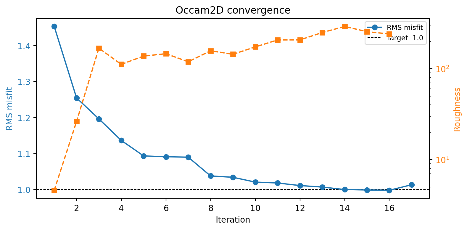
RMS drops steadily from 1.45 toward the target of 1.0 through iteration 14-16, while roughness climbs the entire time as the regularization lets the model depart further from the near-uniform starting half-space. The uptick at iteration 17 is the same non-monotonic step called out in Log And Convergence: RMS got very slightly worse on the very last iteration even as roughness kept rising.

result.plot_model() alone shows the full mesh depth (6 km here), which buries the near-surface structure in a couple of screen pixels. Passing depth_max crops the view to where the interesting structure actually is, and since PlotModel only marks stations with unlabelled triangles, station names can be added afterward directly on the returned Axes.

PlotModel also centers its x-axis on the mesh’s own cell-center mean, not on the stations. This particular mesh has padding on only one side – it reaches 1.82 km past the last station, S46, but 0 km past the first, S00 – so the mesh mean sits about 665 m (roughly 13 average station-spacings) to the right of the stations’ own mean. The practical effect is a profile that reads as shifted toward the padding-heavy side. Re-centering on the stations instead means shifting the pcolormesh image by that same offset, using an affine transform so the resistivity image itself moves rather than being redrawn:

>>> import matplotlib.transforms as mtransforms
>>> from pycsamt.models.occam2d import PlotModel

>>> plotter = PlotModel(result, depth_max=1000.0, figsize=(14, 6.5))
>>> fig = plotter.plot()
>>> ax = fig.axes[0]

>>> cell_centers = (result.mesh.x_nodes[:-1] + result.mesh.x_nodes[1:]) / 2.0
>>> x_shift_mesh = float(cell_centers.mean())
>>> x_shift_station = float(result.data.offsets.mean())
>>> delta_km = (x_shift_mesh - x_shift_station) / 1000.0
>>> print(round(delta_km, 4))
0.6651

>>> quad = ax.collections[0]  # the pcolormesh image
>>> quad.set_transform(mtransforms.Affine2D().translate(delta_km, 0) + ax.transData)

>>> station_x = ax.lines[0].get_xdata() + delta_km  # shift the triangles too
>>> ax.lines[0].set_xdata(station_x)

>>> xlo, xhi = ax.get_xlim()  # follow the same shift -- a transform alone
>>> ax.set_xlim(xlo + delta_km, xhi + delta_km)  # does not move the view

>>> ylo, _ = ax.get_ylim()               # (1004.0, 0.0): depth axis is inverted
>>> for x, name in zip(station_x, result.data.sites):
...     ax.text(x, -0.06 * ylo, name, rotation=90, ha="center", va="bottom",
...             fontsize=6, rotation_mode="anchor")
>>> ax.set_ylim(ylo, -0.22 * ylo)         # reserve headroom for the labels

Two things are easy to miss here. First, rotated text is anchored on its unrotated bounding box unless told otherwise, which visibly shifts 90-degree labels off to one side of the point they are meant to mark; rotation_mode="anchor" applies ha/va after rotation instead, so each label lines up exactly above its triangle. Second, a transform only changes where an artist is drawn – it does not touch the axes’ own view limits, so without explicitly shifting xlim by the same delta_km the view keeps showing the old, unshifted window: part of the resistivity image would run off the right edge while a blank gap opens up on the left where the mesh used to be. The full mesh width – padding included – stays visible; only the coordinate the profile is centered on changes.

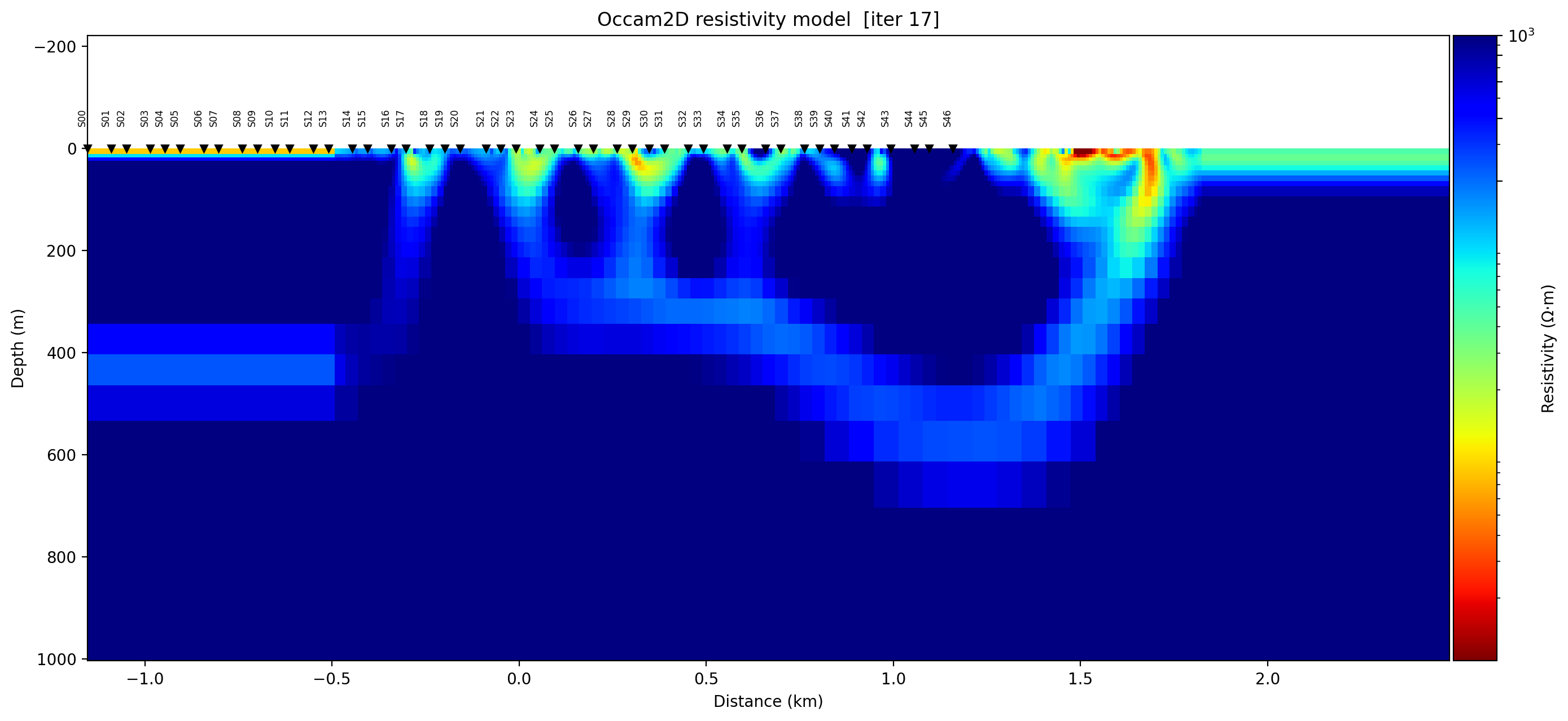
The same model as before, cropped to 1 km depth instead of the full 6 km mesh, re-centered on the stations rather than on the mesh’s own padding-skewed mean, and still showing the full mesh width on both sides – nothing is cropped out. A series of separate near-surface conductive fingers (green/yellow, mostly above 100-300 m) sit under stations S16 through roughly S42, with S00-S15 and S43-S46 over resistive background, and the wide resistive margin to the right of S46 is visibly mesh padding rather than surveyed ground. That asymmetry – padding on one side only – is worth checking with real numbers rather than assumed away, exactly the “is the mesh far wider than the interpreted target” question from Mesh And Model Review.

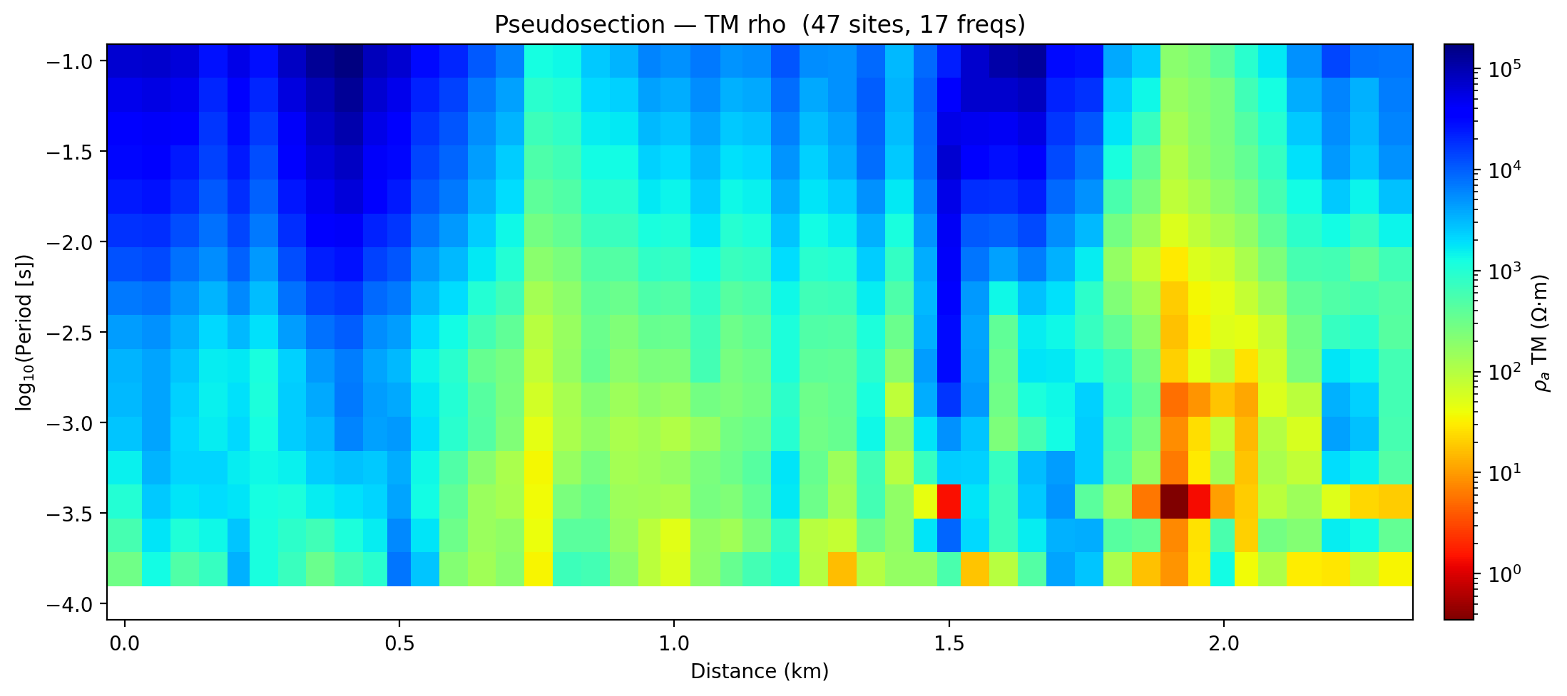
The observed-data pseudosection this model is trying to fit. Two near-surface, short-period low-resistivity patches stand out around 1.5 km and 1.9-2.0 km distance – worth checking against the model section above for static-shift-like artefacts before they are interpreted geologically.

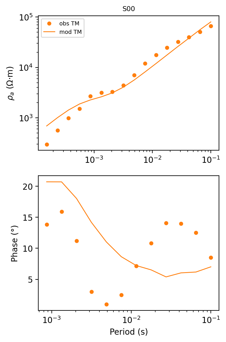
Station S00 in isolation via plot_response(stations=["S00"]). The apparent-resistivity fit (top) is close across the whole period range, but the phase fit (bottom) is not: the smooth model traces a gentle decline while the observed phase scatters between roughly 1 deg and 16 deg with no trend the model reproduces. A coherent resistivity section with a poor phase fit like this one is not, by itself, reliable geological evidence.

PlotResponseGrid scans several stations at once instead of one figure per station. Its per-panel title RMS reads [n/a] for every station in this sample, because the title is computed from obs/pred/error columns inside the response file, and this particular .resp file’s error column is all zero – there is nothing to divide by. response.misfit_per_site() from the previous section reads the same file’s own precomputed weighted residual column instead, which is real and usable, so the two numbers can be patched into the titles after the figure is built:

>>> from pycsamt.models.occam2d import PlotResponseGrid

>>> stations = result.data.sites[:8]
>>> n_cols = 4
>>> fig = PlotResponseGrid(result, stations=stations, n_cols=n_cols).plot()

>>> rms_by_site = result.response.misfit_per_site()
>>> for si, name in enumerate(stations):
...     pg_row, col = divmod(si, n_cols)
...     ax_rho = fig.axes[(2 * pg_row) * n_cols + col]  # top axes of the pair
...     rms_val = rms_by_site.get(si + 1)                # 1-based site index
...     ax_rho.set_title(f"{name}  [{rms_val:.2f}]", fontsize="xx-small")

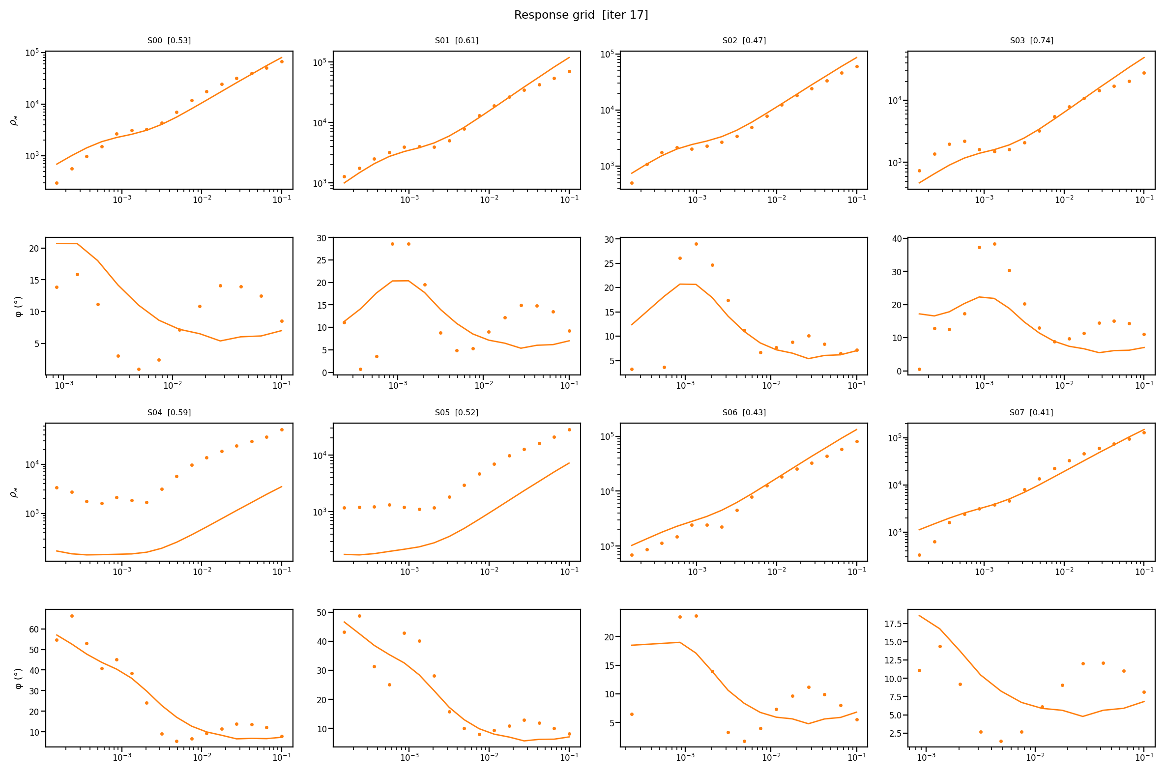
Fit quality is clearly uneven across the profile: S00-S03, S06, and S07 track the model reasonably well in apparent resistivity, while S04 and S05 sit an order of magnitude below the model curve at short period. What is not obvious from the plots alone is that S04 (RMS 0.59) and S05 (RMS 0.52) are not the worst-fitting stations here – S03 is (RMS 0.74), despite tracking the observed resistivity closely. Occam’s weighted residual mixes rho and phase rows for the whole period range into one number per site, so a single per-site RMS can still hide exactly which component or period band is driving the misfit; the grid of curves is what actually shows that, not the number in the title.

Before interpretation, compare the section against residual plots. A coherent anomaly with poor response fit is not reliable geological evidence.

6.2.5.14. Recommended Run Layout

Keep one run directory per scientific experiment.

runs/
  profile_a_occam2d_v01/
    occam2d.yml
    provenance.yml
    native/
      OccamDataFile.dat
      Occam2DMesh
      Occam2DModel
      Startup
      ITER17.iter
      RESP17.resp
      LogFile.logfile
      occam_stdout.log
      occam_stderr.log
    qc/
      pseudosection.png
      convergence.png
      response_fit_site_S00.png
      section_iter17.png
    exports/
      profile_a_iter17.dat
      run_snapshot.zip

Avoid launching new experiments in an old output directory. Occam-style native files often have simple names, and stale .iter or .resp files can be mistaken for fresh output.

6.2.5.15. Pre-Run Checklist

Before launching:

• load OccamConfig from the edited template;

• confirm station order and profile offsets;

• inspect selected modes and frequency band;

• confirm apparent-resistivity and phase error floors;

• inspect mesh dimensions, padding, and depth growth;

• inspect model parameter count;

• confirm startup file references the intended data, mesh, and model files;

• confirm the executable path and compiler provenance;

• move old iteration, response, and log files out of the native directory;

• record the exact command and runtime environment.

6.2.5.16. Post-Run Checklist

After completion:

• read stdout/stderr logs if pyCSAMT launched the run;

• load the run with InversionResult;

• confirm the selected iteration number and final RMS;

• inspect convergence history, and compare it against the selected .iter file’s own misfit value rather than assuming they agree;

• inspect per-site and per-frequency misfit;

• compare observed and modeled responses;

• plot the pseudosection and final model together;

• export iter2dat only after confirming the selected iteration;

• archive the native input and output files with the configuration.

6.2.5.17. Common Mistakes

Interpreting smooth gradients too literally

Occam regularization intentionally smooths structure. A gradient may represent a sharper geological contact that is not resolved by the data.

Ignoring station geometry

The data, mesh, pseudosection, and model section all depend on station ordering and offsets. Check them before running.

Using unrealistic error floors

Too-small floors can force the inversion to fit noise; too-large floors can underfit useful signal.

Mixing old and new output files

If a run fails, old .iter or .resp files can remain. Check timestamps and log files before loading.

Forgetting startup patching

Passing max_iter or target_misfit to OccamRunner.run modifies Startup in place. Archive the modified file.

Passing plotting keywords by guesswork

plot_response takes stations=[...], not site=.... An unknown keyword is silently absorbed rather than rejected, so the plot still renders – just not the one that was asked for. Check the keyword names in the API reference rather than assuming an argument name.

Trusting one backend_options key without checking the adapter

The Occam2D backend reads native settings from backend_options["config"]. Any other key name is ignored, and the run silently falls back to OccamConfig() defaults with no warning.

6.2.5.18. Next Steps

• Configuration And File I/O for source-of-truth configuration and native file archive practice.

• Compiling the External Solvers builds Occam2D from the vendored source, on Windows, Linux, or macOS.

• Choosing A Model Backend for deciding when Occam2D is the right model integration.

• Prepare an Occam2D Inversion for a practical Occam2D workflow.

• Inversion Concepts for Occam-style objective functions and regularization.

• pycsamt.models for generated API details.