
16.1. Overview#
16.1.1. Forward And Model Integrations#
The pycsamt.forward and pycsamt.models packages are related, but
they should not be treated as the same layer.
Package |
Main responsibility |
Typical use |
|---|---|---|
Compute controlled forward responses inside Python using pyCSAMT model containers, solvers, dataset generators, noise models, and plotting helpers. |
Test survey design, generate training data, validate inversion assumptions, compare response behaviour, and build reproducible synthetic examples. |
|
Integrate external modelling and inversion engines such as Occam2D, ModEM, and MARE2DEM. |
Prepare native engine files, run external binaries, load engine outputs, and manage backend-specific inversion projects. |
Use pycsamt.forward when you need a controlled synthetic dataset
or response from a known model. Use pycsamt.models when you need to
prepare, run, or load a native external-engine project. The two layers meet
when a forward synthetic experiment is converted into an inversion benchmark:
the known model gives the reference answer, and the inversion workflow tests
whether that answer can be recovered from the predicted data.
16.1.2. Package Map#
The public forward API is built around a small set of object families.
Object family |
Main objects |
Role |
|---|---|---|
Configuration |
|
Store reproducible frequency/time axes, model ranges, station layouts, solver options, noise settings, and output choices. |
Model containers |
|
Represent 1-D layered earths, 2-D profile grids, and quasi-3-D resistivity volumes. |
Solvers |
|
Compute predicted electromagnetic responses from model containers. |
Response containers |
|
Hold predicted apparent resistivity, phase, transient values, impedance tensor components, survey geometry, and array conversion helpers. |
Noise models |
|
Convert ideal synthetic responses into more realistic observations. |
Dataset containers |
|
Store synthetic feature and target arrays, metadata, splits, and
compressed |
Plotting helpers |
|
Inspect models, responses, tensor components, noisy examples, and generated datasets before they are trusted downstream. |
16.1.3. Core Workflow#
A typical forward modelling workflow has six stages. The smallest version starts with a 1-D layered earth because the geometry is easy to audit: resistivity is a function of depth only, \(\rho=\rho(z)\), and the MT solver predicts the impedance \(Z(f)\) for each frequency. The reported curves are then derived in the usual way from impedance magnitude and phase, with apparent resistivity proportional to \(|Z|^2/f\). In other words, the model is compact, but the response still carries the frequency-dependent signature that an inversion or interpretation workflow would need.
 1>>> import numpy as np
 2
 3>>> from pycsamt.forward import LayeredModel, MT1DForward, plot_response_and_model_1d
 4
 5>>> freqs = np.logspace(-2, 3, 40)
 6>>> model = LayeredModel(
 7...     resistivity=[100.0, 15.0, 800.0],
 8...     thickness=[250.0, 700.0],
 9... )
10
11>>> solver = MT1DForward(freqs)
12>>> response = solver.run(model)
13>>> print(f"response: {response.method}, {response.freqs.size} frequencies")
14response: MT1D, 40 frequencies
15>>> print(f"rho_a range: {response.rho_a.min():.2f}-{response.rho_a.max():.2f} Ohm.m")
16rho_a range: 20.57-475.29 Ohm.m
17>>> print(f"phase range: {response.phase.min():.2f}-{response.phase.max():.2f} deg")
18phase range: 18.14-61.70 deg
19
20>>> fig = plot_response_and_model_1d(response, model)
21>>> fig.savefig("runs/forward/mt1d_response.png", dpi=200)
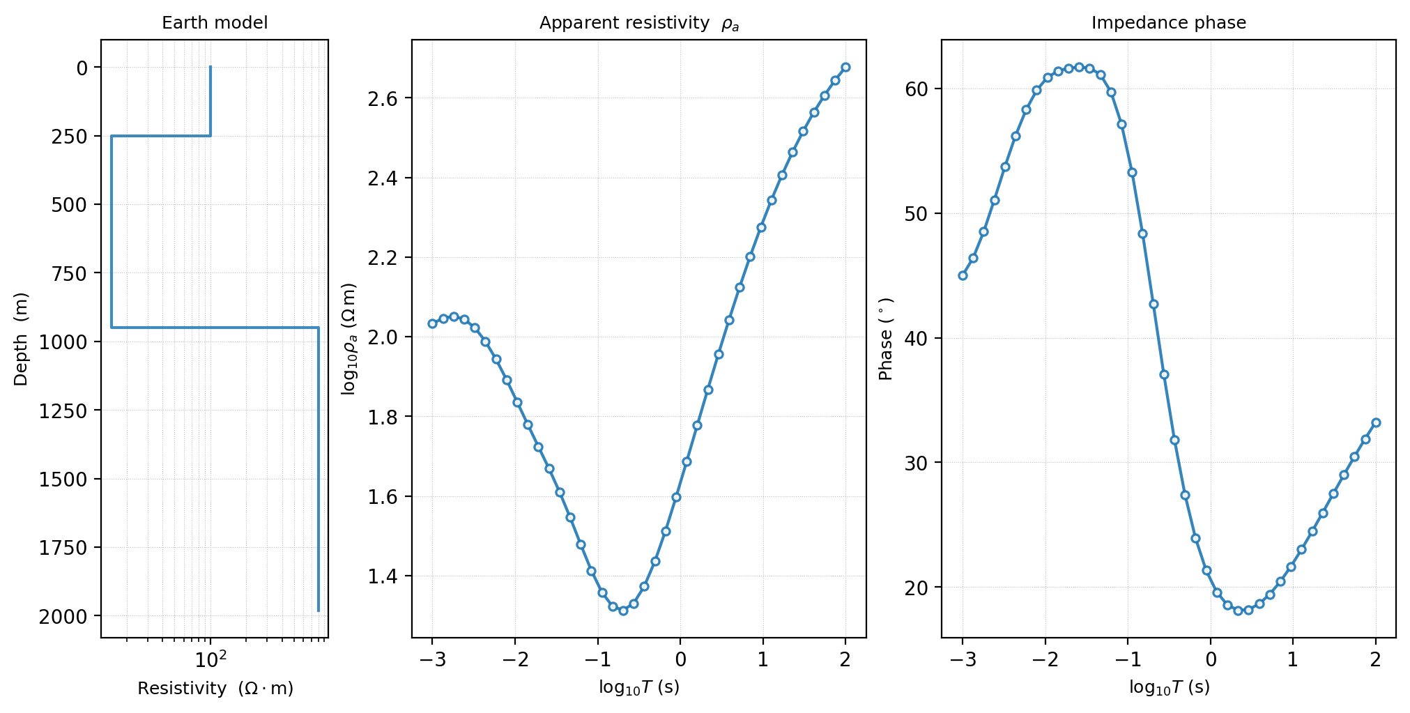
A three-layer MT1D example generated from the code above. The conductive middle layer lowers \(\rho_a\) over part of the period range, while the phase curve records the transition between layers.#
For production work, the same idea should be driven by a configuration file and archived with outputs:
define the physical question and target dimensionality;
create a
ForwardConfig*template;build a model or grid from the configuration;
run the selected solver;
apply a documented noise model when simulating observations;
plot and archive the model, response, configuration, and metadata.
ForwardConfig is the object that carries stages 1-2
and part of stage 5: it records the sampled frequency grid (or
time gate grid for TEM), the solver name, and the noise settings that
a collaborator would need to reproduce the run, rather than leaving them
scattered across a script. Forward Configuration covers all three
ForwardConfig* classes, template files, and validation in depth; the
compact version below only threads a single config through stages 3-5 for
the same three-layer model as above, this time with a documented noise model
applied.
 1>>> from pycsamt.forward import (
 2...     ForwardConfig, LayeredModel, MT1DForward, GaussianNoise,
 3...     plot_response_and_model_1d,
 4... )
 5
 6>>> cfg = ForwardConfig(
 7...     solver="mt1d", freq_min=1e-2, freq_max=1e3, n_freqs=40,
 8...     noise_level=0.05, seed=0,
 9... )
10>>> cfg.validate()
11>>> freqs = cfg.freq_grid()
12>>> print(f"freqs: {freqs.size} points, {freqs.min():.2e}-{freqs.max():.2e} Hz")
13freqs: 40 points, 1.00e-02-1.00e+03 Hz
14
15>>> model = LayeredModel(resistivity=[100.0, 15.0, 800.0], thickness=[250.0, 700.0])
16>>> clean = MT1DForward(freqs).run(model)
17>>> noisy = GaussianNoise(level=cfg.noise_level).apply(clean, seed=cfg.seed)
18>>> print(f"clean rho_a[0] = {clean.rho_a[0]:.2f} Ohm.m, noisy rho_a[0] = {noisy.rho_a[0]:.2f} Ohm.m")
19clean rho_a[0] = 475.29 Ohm.m, noisy rho_a[0] = 482.22 Ohm.m
20>>> print(f"clean phase[0] = {clean.phase[0]:.2f} deg, noisy phase[0] = {noisy.phase[0]:.2f} deg")
21clean phase[0] = 33.22 deg, noisy phase[0] = 30.39 deg
22
23>>> fig = plot_response_and_model_1d(noisy, model, title="Noisy MT1D response (5% Gaussian)")
24>>> fig.savefig("runs/forward/mt1d_noisy_response.png", dpi=200)
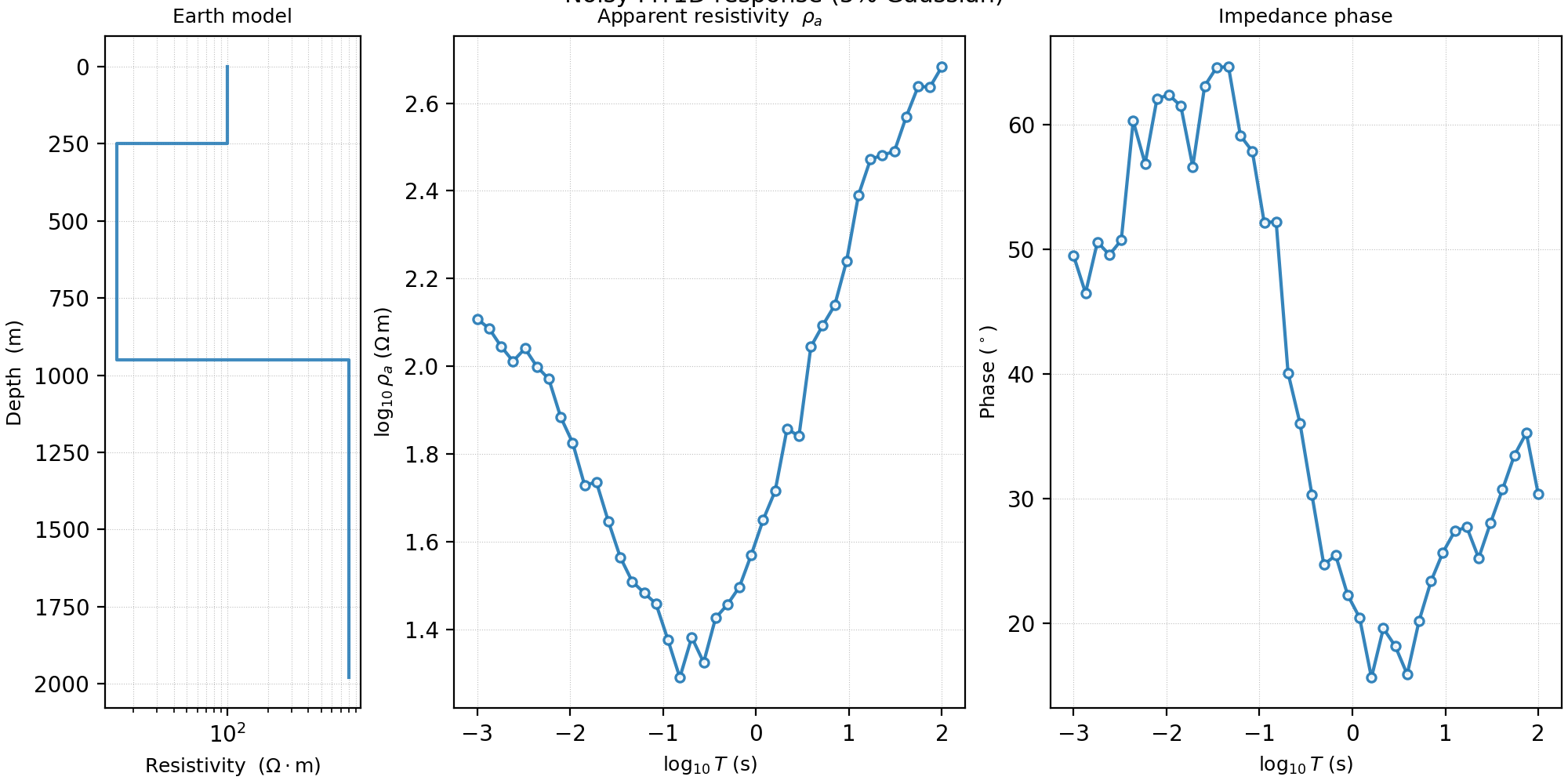
Same three-layer model, now with a noise model applied to
\(\rho_a\) and phase independently, seeded for reproducibility.
noise_level=0.05 is a standard deviation in
\(\log_{10}\rho_a\)-space, not a direct linear-relative percentage –
for this seeded draw the realized linear relative scatter in
\(\rho_a\) across all 40 points has a standard deviation of about 9.0%
(largest single deviation 23%), and phase scatter has a standard
deviation of about 2.4° (matching the default phase_level =
noise_level * 45). Neither shows any systematic dependence on period –
each frequency’s perturbation is drawn independently, so the noisiest
point in a given realization is wherever the random draw happened to land
largest, not a fixed feature of the curve.#
Both examples share the same physical model and solver; the difference is entirely in what gets carried forward for someone else to reproduce. The first is fine for a quick, throwaway check. The second – config, seed, and noise level all explicit and archivable – is the version worth keeping in a project.
16.1.4. Choosing A Path#
Different users enter the forward section with different goals.
Goal |
Start here |
Then read |
|---|---|---|
Understand the physics and vocabulary |
||
Build a reproducible synthetic run |
||
Generate training data for AI inversion |
Forward Configuration, Forward Plotting, AI And Model-Zoo Agents |
|
Compare 1-D, 2-D, and quasi-3-D behaviour |
||
Prepare an inversion benchmark |
||
Diagnose a generated dataset or response |
Synthetic Datasets And Noise, From Forward Modelling To Inversion |
|
Get a response with a checkable accuracy claim, or a production-backed forward check |
16.1.5. Relationship To Theory#
Forward modelling is practical, but it is not detached from theory. When a plot or synthetic response looks surprising, the relevant background pages are:
CSAMT, AMT, and MT Overview for the distinction between CSAMT, AMT, MT, and TEM survey assumptions;
Impedance Tensor for impedance, apparent resistivity, phase, and tensor notation;
Static Shift for shallow distortion effects that can make synthetic and field curves disagree;
Inversion Concepts for how forward responses are used inside objective functions and regularized inversion.