6.1. Overview

6.1.1. Before Any Inversion

Do not start with a solver. Start with evidence that the data and modelling assumptions are suitable. A reproducible inversion package should retain:

• the EDI or processed observation source and the exact processing steps;

• frequency/period band, components, units, station order, and coordinates;

• QC tables, confidence decisions, and any frequencies recovered or masked;

• static-shift, noise-removal, tensor-rotation, and dimensionality evidence;

• error floors or uncertainty model, with justification;

• chosen dimensionality: 1-D sounding, stitched 2-D profile, true 2-D, 2.5-D, or 3-D;

• starting model, bounds, regularization, mesh/grid, and covariance controls;

• executable identity for external solvers and whether external execution was explicitly requested;

• residual, convergence, response-fit, and model-appraisal products.

Useful preparation pages are EM Tools Guide, Dimensionality Assessment, Choosing A Model Backend, and Inversion Concepts.

6.1.2. Backend-Neutral Workflow

pycsamt.inversion separates configuration, execution, results, and export:

InversionConfig

Describes method, dimension, backend, data arrays, starting model, solver limits, error settings, backend options, and output policy.

InversionWorkflow

Resolves the selected backend and runs the workflow. For external engines, execution remains explicit through the backend configuration.

InversionResult

Stores recovered model values, diagnostics, uncertainty, history, native files, and conversion helpers such as to_resistivity_model().

pycsamt.inversion.export and pycsamt.inversion.plot

Write common products and quick-look figures from a result object.

At a glance, backend names accepted by the common API include:

Backend	Main use	Notes
builtin	Lightweight local inversion	MT/AMT/CSAMT layered 1-D, TDEM 1-D, stitched 2-D profiles, and optional finite-difference 2-D profile experiments.
occam2d	Smooth 2-D profile inversion	Prepares/validates native Occam2D files and can run an external executable when configured.
modem	2-D or 3-D ModEM workflow	Manages native ModEM data/model/control/covariance conventions and completed-run loading.
simpeg	Optional SimPEG adapter	Imported only when selected and installed.
pygimli	Optional pyGIMLi adapter	Useful for 1-D EM modelling/inversion and stitched profile experiments.

MARE2DEM is documented under MARE2DEM. It is a rich native model integration for 2.5-D MT/CSEM projects; use it directly when the MARE2DEM file set and finite-element workflow are the scientific target.

6.1.3. Minimal MT 1-D

This synthetic example uses the built-in backend so it can run without an external solver:

>>> import numpy as np
>>> from pycsamt.forward import LayeredModel, MT1DForward
>>> from pycsamt.inversion import (
...     InversionConfig,
...     InversionWorkflow,
...     StartingModel,
... )

>>> freqs = np.logspace(-2, 2, 12)
>>> truth = LayeredModel([80.0, 25.0, 600.0], [250.0, 900.0])
>>> response = MT1DForward(freqs=freqs).run(truth)

>>> cfg = InversionConfig(
...     method="mt",
...     dimension="1d",
...     backend="builtin",
...     data={
...         "freqs": freqs,
...         "rho_a": response.rho_a,
...         "phase": response.phase,
...     },
...     starting_model=StartingModel(
...         resistivities=[100.0, 50.0, 500.0],
...         thicknesses=[300.0, 1000.0],
...     ),
...     max_iter=12,
... )

>>> result = InversionWorkflow(cfg).run()
>>> print(result.summary())
InversionResult(method='mt', dimension='1d', backend='builtin', status='converged', rms=9.21e-15)

The RMS here is essentially zero because the “observations” are noiseless forward responses of a known truth model with the built-in inversion started from a nearby model – a sanity check, not a realistic field result. Treat this as confirmation that the round trip (forward model -> inversion -> recovered model) works, not as evidence about real-world convergence.

6.1.4. Minimal TDEM 1-D

The same pattern works for TDEM when the data vector is a time-domain decay:

>>> import numpy as np
>>> from pycsamt.forward import LayeredModel, TEM1DForward
>>> from pycsamt.inversion import (
...     InversionConfig,
...     InversionWorkflow,
...     StartingModel,
... )

>>> times = np.logspace(-5, -3, 7)
>>> truth = LayeredModel([60.0, 250.0, 900.0], [120.0, 700.0])
>>> forward_options = {"loop_radius": 25.0, "n_freqs": 10, "n_lam": 16}
>>> response = TEM1DForward(times=times, **forward_options).run(truth)

>>> cfg = InversionConfig(
...     method="tdem",
...     dimension="1d",
...     backend="builtin",
...     data={"times": times, "values": response.dBz_dt},
...     starting_model=StartingModel(
...         resistivities=[80.0, 200.0, 700.0],
...         thicknesses=[150.0, 800.0],
...     ),
...     backend_options=forward_options,
...     max_iter=8,
... )

>>> result = InversionWorkflow(cfg).run()
>>> print(result.summary())
InversionResult(method='tdem', dimension='1d', backend='builtin', status='needs_review', rms=3.83)

Unlike the noiseless MT case above, this TDEM run reports needs_review with rms=3.83 – a real (if extreme) illustration of why summary() and status must be checked rather than assumed. Seven time gates, an 8-iteration cap, and a coarse three-layer starting model are not enough for this synthetic decay to converge; do not treat a returned InversionResult as a fitted model until its status and RMS have been reviewed.

6.1.5. Profile Inversion

For a profile where each station has responses on a common frequency grid, pass station-by-frequency arrays. Continuing the fixture above with two more stations built the same way (rho_by_station/phase_by_station stacked as (n_stations, n_frequencies) arrays from three nearby LayeredModel truths):

>>> cfg = InversionConfig(
...     method="mt",
...     dimension="2d",
...     backend="builtin",
...     data={
...         "freqs": freqs,
...         "rho_a": rho_by_station,      # (n_stations, n_frequencies)
...         "phase": phase_by_station,    # (n_stations, n_frequencies)
...         "station_x": [0.0, 400.0, 800.0],
...         "station_names": ["S00", "S01", "S02"],
...     },
...     starting_model=StartingModel(
...         resistivities=[100.0, 50.0, 600.0],
...         thicknesses=[300.0, 900.0],
...     ),
...     max_iter=10,
... )
>>> result = InversionWorkflow(cfg).run()
>>> print(result.summary())
InversionResult(method='mt', dimension='2d', backend='builtin', status='success', rms=1.48e-09)
>>> model = result.to_resistivity_model()
>>> model.rho_2d.shape
(3, 3)

to_resistivity_model() gives a pycsamt.interp.ResistivityModel with one column per station and one row per starting-model layer – here (3, 3) for three stations and the three-layer StartingModel. This is the same conversion used throughout Interpretation workflow.

The built-in dimension="2d" path may represent either stitched station inversions or an opt-in finite-difference profile experiment, depending on backend_options:

>>> cfg.backend_options.update(
...     {
...         "profile_mode": "fd2d",
...         "nx": 12,
...         "n_pad": 2,
...         "components": ("te", "tm"),
...     }
... )

Updating backend_options alone does not re-run the inversion; call InversionWorkflow(cfg).run() again to fit the fd2d profile experiment.

For production smooth 2-D profile inversion, review Occam2D. For 3-D MT/AMT projects, review ModEM. For 2.5-D MT/CSEM finite-element projects, review MARE2DEM.

6.1.6. Exports And Review

All common export helpers accept an InversionResult:

>>> from pycsamt.inversion import export, plot

>>> export.to_csv(result_2d, "model.csv")
>>> export.to_npz(result_2d, "model.npz")
>>> export.to_geojson(result_2d, "model.geojson")
>>> export.to_vtk(result_2d, "model.vtk")
>>> export.to_archive(result_2d, "snapshot.zip")

>>> # Requires rasterio.
>>> export.to_geotiff(result_2d, "model.tif")

>>> ax = plot.plot_model(result_2d, savepath="model.png")
>>> ax = plot.plot_rms(result_2d, savepath="rms.png")

Both plot_model and plot_rms return the matplotlib Axes they drew into, not a Figure; get the figure back with ax.figure if you need it (for example, to call fig.savefig yourself instead of the savepath argument). For the three-station profile result from above:

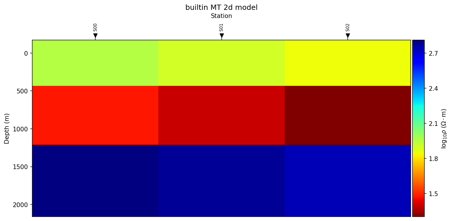
plot.plot_model(result_2d) – the recovered log10-resistivity section, station markers included.

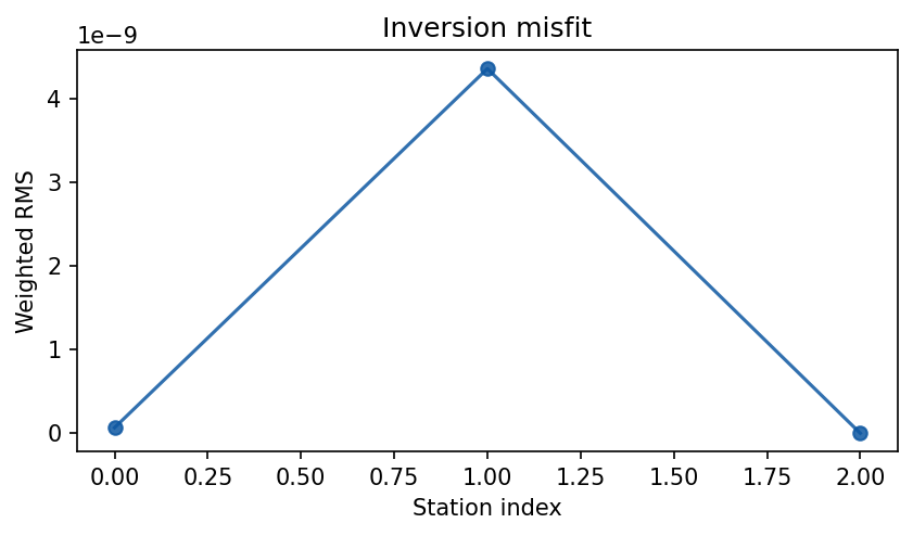
plot.plot_rms(result_2d) – one marker per station, because the builtin backend’s stitched-station 2-D path populates result.metadata["station_rms"]. Without that key, plot_rms falls back to a single global bar from result.rms.

Archive the configuration and review products together with these exports. The final color section is not enough for scientific reproducibility.

6.1.7. Hydrogeophysical Handoff

Any inversion result that can be converted to ResistivityModel can enter the pycsamt.interp hydrogeophysical workflow:

>>> from pycsamt.interp import EMHydroModel, PetrophysicalConfig
>>> from pycsamt.interp.petrophysics import ArchieModel

>>> resistivity_model = result_2d.to_resistivity_model()
>>> hydro_cfg = PetrophysicalConfig(
...     petro=ArchieModel(m=1.8, n=2.0),
...     rho_w=20.0,
...     porosity_prior=0.28,
... )
>>> hydro = EMHydroModel(resistivity_model, hydro_cfg, method_tag="MT").fit()
>>> print(hydro.water_table)
[130. 130. 130.]

The three-layer starting model used above only has three depth cells, so the handoff here is illustrative rather than a realistic hydrogeophysical section – see Hydrogeophysical interpretation for the full audit and validation steps to apply before trusting a water-table detection like this one.

6.1.8. Next Steps

Use these pages depending on the work in front of you:

• Classical model integrations for classical Occam2D, ModEM, and MARE2DEM projects.

• Choosing A Model Backend before committing to a solver.

• Inversion Concepts for objective functions, RMS, regularization, uncertainty, resolution, and non-uniqueness.

• AI inversion for learned inversion workflows.

• Interpretation when moving from a model to geological or hydrogeophysical interpretation.

• Inversion for runnable gallery examples.